7.12. The Levenberg-Marquardt Method#
The Levenberg-Marquardt (LM) method is an optimization algorithm used to solve non-linear least-squares problems. The LM method finds the model parameters \(\boldsymbol{\theta}\) that minimize the residual sum of squares
where \(y_i\) represents the observed data, \(f\) is a non-linear model function, \(\mathbf{x}_i\) denotes the corresponding predictive variables, and \(r_i = y_i - f(\boldsymbol{\theta}, \mathbf{x}_i)\) is the residual. For these notes, lete \(N\) be the number of data points, so that \(i=1, 2, ..., N\) and \(n\) be the number of model parameters.
The LM algorithm acts as an adaptive interpolation between gradient descent and Gauss-Newton iteration. Consequently, to understand the LM method, we first cover Gauss-Newton iteration.
The Gauss-Newton iteration updates the model parameters by \(\boldsymbol{\theta} \to \boldsymbol{\theta} + \boldsymbol{\Delta\theta}\), where the update \(\boldsymbol{\Delta\theta}\) is chosen by minimizing a linearized version of the loss. Let \(\mathbf{J}\) denote the Jacobian of the model with respect to the parameters, with entries
so that \(\mathbf{J}\) has \(N\) rows, one per data point, and \(n\) columns, one per parameter. A first-order Taylor expansion of the model around \(\boldsymbol{\theta}\) gives \(f(\boldsymbol{\theta} + \boldsymbol{\Delta\theta}, \mathbf{x}_i) \approx f(\boldsymbol{\theta}, \mathbf{x}_i) + \sum_j J_{ij} \Delta\theta_j\), and because the observed data \(y_i\) are constants the residual vector expands as \(\mathbf{r}(\boldsymbol{\theta} + \boldsymbol{\Delta\theta}) \approx \mathbf{r}(\boldsymbol{\theta}) - \mathbf{J}\boldsymbol{\Delta\theta}\). The approximate loss \(L(\boldsymbol{\theta} + \boldsymbol{\Delta\theta}) \approx \frac{1}{2}\|\mathbf{r} - \mathbf{J}\boldsymbol{\Delta\theta}\|^2\) is quadratic in \(\boldsymbol{\Delta\theta}\), so finding the update that minimizes it is an ordinary linear least-squares problem. We now derive that statement.
Substituting the linearized model into the loss function yields
To find the update vector \(\boldsymbol{\Delta\theta}\) that minimizes this quadratic approximation, we set the partial derivative of \(L\) with respect to each component \(\Delta\theta_k\) to zero,
Note, since \(\boldsymbol{\theta}\) is held fixed, the update \(\boldsymbol{\Delta\theta}\) is the only variable in the approximation, and setting \(\partial L/\partial \Delta\theta_k = 0\) is the same condition we would impose to locate a minimum at the point \(\boldsymbol{\theta} + \boldsymbol{\Delta\theta}\).
Expanding the product and collecting the terms that contain \(\Delta\theta_j\) on the left-hand side gives
Interchanging the order of summation on the left-hand side pulls the parameter updates \(\Delta\theta_j\) outside the sums over the data,
The inner sum on the left is the \((k,j)\) element of \(\mathbf{J}^T\mathbf{J}\) and the right-hand side is the \(k\)-th element of \(\mathbf{J}^T\mathbf{r}\), so the system of \(n\) linear equations above is the normal equations
Solving for the update vector yields the Gauss-Newton step
The inverse in the equation above is written for clarity and is not formed in practice. The matrix \(\mathbf{J}^T\mathbf{J}\) is symmetric positive semi-definite, so when \(\mathbf{J}\) has full column rank the normal equations can be solved by Cholesky decomposition, and solving the linear least-squares problem by QR decomposition of \(\mathbf{J}\) avoids forming \(\mathbf{J}^T\mathbf{J}\) altogether at the cost of squaring the condition number.
Gauss-Newton fails in two ways. If \(\mathbf{J}\) loses full column rank, which happens when two parameters have nearly the same effect on the model or when a parameter barely affects the model at all, then \(\mathbf{J}^T\mathbf{J}\) is singular or ill-conditioned and the step is either undefined or enormous. Even with a well-conditioned \(\mathbf{J}\), the step is computed from a linearization that is only accurate near \(\boldsymbol{\theta}\), so a large step can overshoot and increase the loss. The Levenberg-Marquardt method addresses both failures by adding a damping term to \(\mathbf{J}^T\mathbf{J}\).
7.12.1. Levenberg’s Contribution: Damped Least Squares#
Gauss-Newton fails when \(\mathbf{J}^T\mathbf{J}\) is singular or ill-conditioned, which produces enormous steps, and it fails when the linearization is poor, which produces steps that overshoot and increase the loss. In 1944, Kenneth Levenberg addressed both problems by adding a non-negative damping parameter \(\lambda \ge 0\) to the diagonal of the normal equations,
The eigenvalues of \(\mathbf{J}^T\mathbf{J} + \lambda\mathbf{I}\) are \(\sigma_j^2 + \lambda\), where the \(\sigma_j\) are the singular values of \(\mathbf{J}\), so for \(\lambda > 0\) the matrix is positive definite even when \(\mathbf{J}\) is rank deficient. The system always has a unique solution and the step is always a descent direction.
7.12.1.1. Transitioning Between Gradient Descent and Gauss-Newton#
The size of \(\lambda\) controls how the update interpolates between gradient descent and the Gauss-Newton step.
For large damping, \(\mathbf{J}^T\mathbf{J} + \lambda\mathbf{I} \approx \lambda\mathbf{I}\) and the update reduces to
a small step along the steepest descent direction. This is the safe regime, used when the estimate is far from the minimum or the linearization is poor.
For small damping, the damping term vanishes and the update reduces to the undamped Gauss-Newton step
which converges rapidly near the minimum.
7.12.2. Approximating the Hessian#
The Gauss-Newton step is Newton-like because \(\mathbf{J}^T\mathbf{J}\) approximates the Hessian of the loss. Starting from \(L(\boldsymbol{\theta}) = \frac{1}{2}\sum_i (y_i - f(\boldsymbol{\theta},\mathbf{x}_i))^2\), the first derivative with respect to \(\theta_k\) is
and differentiating again with respect to \(\theta_l\) yields
In matrix form the exact Hessian is
The Gauss-Newton approximation drops the second term, which is small for either of two reasons. The residuals \(r_i\) are small near a good fit, or the model \(f\) is nearly linear near \(\boldsymbol{\theta}\) so that \(\nabla^2 f\) is negligible. Dropping the term gives \(\nabla^2 L(\boldsymbol{\theta}) \approx \mathbf{J}^T\mathbf{J}\) and avoids computing second derivatives of the model.
The same condition governs convergence speed. Gauss-Newton converges quadratically when the residuals vanish at the solution, and only linearly otherwise, at a rate set by the size of the dropped term relative to \(\mathbf{J}^T\mathbf{J}\).
Below a from-scratch LM method is used to fit the three-parameter model \(f(\boldsymbol{\theta}, x) = \theta_0 e^{-\theta_1 x} + \theta_2\) to synthetic data generated from \(\boldsymbol{\theta}_\mathrm{true} = (5.0, 1.2, 0.5)\) with Gaussian noise of standard deviation \(0.05\) added to each point. The Jacobian is computed analytically, with columns \(\partial f/\partial\theta_0 = e^{-\theta_1 x}\), \(\partial f/\partial\theta_1 = -\theta_0 x e^{-\theta_1 x}\), and \(\partial f/\partial\theta_2 = 1\). The initial guess \(\boldsymbol{\theta}_0 = (2.0, 0.5, 0.0)\) is deliberately far from the true parameters so that the early iterations exercise the damped regime.
A trial and error approach is used to determine the damping parameter \(\lambda\). At each iteration the damped normal equations are solved for \(\boldsymbol{\Delta\theta}\) and the loss is evaluated at the trial point \(\boldsymbol{\theta} + \boldsymbol{\Delta\theta}\). If the loss decreased the step is accepted and \(\lambda\) is divided by a factor of ten, which moves the next step toward Gauss-Newton. If the loss increased the step is rejected, \(\boldsymbol{\theta}\) is left unchanged, and \(\lambda\) is multiplied by ten, which shortens the next step and turns it toward steepest descent. Because \(\|\boldsymbol{\Delta\theta}\| \to 0\) as \(\lambda \to \infty\), repeated rejections are guaranteed to produce an acceptable step unless the current \(\boldsymbol{\theta}\) is already a stationary point.
Iteration stops when the gradient \(\mathbf{J}^T\mathbf{r}\) is small, when an accepted step is small, or when \(\lambda\) reaches its upper bound. The step-size test is applied only to accepted steps, since after a rejection a small \(\boldsymbol{\Delta\theta}\) reflects large damping rather than convergence.
import numpy as np

# =====================================================================
# 1. TEST CASE SETUP: 3-Parameter Exponential Decay with Offset
# =====================================================================

# Model: f(x) = theta_0 * exp(-theta_1 * x) + theta_2
theta_true = np.array([5.0, 1.2, 0.5])
x = np.linspace(0, 4, 50)


def model(theta, x):
    return theta[0] * np.exp(-theta[1] * x) + theta[2]


np.random.seed(42)
y_noisy = model(theta_true, x) + np.random.normal(0, 0.05, size=x.shape)


def compute_residuals(theta, x, y):
    """r_i = y_i - f(theta, x_i)"""
    return y - model(theta, x)


def compute_jacobian(theta, x):
    """Model Jacobian with entries J_ij = df(x_i)/d(theta_j)"""
    J = np.zeros((len(x), len(theta)))
    J[:, 0] = np.exp(-theta[1] * x)
    J[:, 1] = -theta[0] * x * np.exp(-theta[1] * x)
    J[:, 2] = 1.0
    return J


# =====================================================================
# 2. LEVENBERG-MARQUARDT SOLVER FROM SCRATCH
# =====================================================================


def levenberg_marquardt(
    x,
    y,
    theta_init,
    lambda_init=1e-2,
    lambda_factor=10.0,
    lambda_bounds=(1e-12, 1e10),
    max_iter=100,
    tol_step=1e-8,
    tol_grad=1e-8,
):
    """Solve non-linear least squares by the Levenberg-Marquardt algorithm."""
    theta = theta_init.copy().astype(float)
    lam = lambda_init
    lam_min, lam_max = lambda_bounds

    r = compute_residuals(theta, x, y)
    loss = 0.5 * np.sum(r**2)
    J = compute_jacobian(theta, x)

    print(f"{'Iter':<5} | {'Loss':<12} | {'Lambda':<10} | {'Parameters':<28} | Status")
    print("-" * 78)
    print(f"{0:<5} | {loss:<12.6f} | {lam:<10.2e} | {str(np.round(theta, 4)):<28} |")

    for i in range(1, max_iter + 1):
        # Gradient of the loss is -J^T r, so J^T r is the descent direction
        gradient = J.T @ r

        if np.max(np.abs(gradient)) < tol_grad:
            print(f"\nConverged in {i - 1} iterations (gradient).")
            break

        # Damped normal equations (J^T J + lambda I) delta_theta = J^T r
        A = J.T @ J + lam * np.eye(len(theta))
        delta_theta = np.linalg.solve(A, gradient)

        theta_trial = theta + delta_theta
        r_trial = compute_residuals(theta_trial, x, y)
        loss_trial = 0.5 * np.sum(r_trial**2)

        if loss_trial < loss:
            # Accept, reduce damping, and refresh the Jacobian at the new theta
            theta, r, loss = theta_trial, r_trial, loss_trial
            J = compute_jacobian(theta, x)
            lam = max(lam / lambda_factor, lam_min)
            status = "Accepted"
            converged = np.linalg.norm(delta_theta) < tol_step
        else:
            # Reject and increase damping. Theta is unchanged, so J is still valid
            lam = min(lam * lambda_factor, lam_max)
            status = "Rejected"
            converged = False

        print(
            f"{i:<5} | {loss:<12.6f} | {lam:<10.2e} | {str(np.round(theta, 4)):<28} | {status}"
        )

        if converged:
            print(f"\nConverged in {i} iterations (step size).")
            break

        if lam >= lam_max:
            print(f"\nStopped at iteration {i}: damping hit upper bound.")
            break

    return theta, loss


# =====================================================================
# 3. RUN SOLVER
# =====================================================================

theta_init = np.array([2.0, 0.5, 0.0])
theta_opt, final_loss = levenberg_marquardt(x, y_noisy, theta_init)

print("\nResults Summary:")
print(f"True Parameters:      {theta_true}")
print(f"Estimated Parameters: {np.round(theta_opt, 4)}")
Iter  | Loss         | Lambda     | Parameters                   | Status
------------------------------------------------------------------------------
0     | 29.548474    | 1.00e-02   | [2.  0.5 0. ]                |
1     | 22.093073    | 1.00e-03   | [3.4383 2.0304 1.8538]       | Accepted
2     | 22.093073    | 1.00e-02   | [3.4383 2.0304 1.8538]       | Rejected
3     | 22.093073    | 1.00e-01   | [3.4383 2.0304 1.8538]       | Rejected
4     | 22.093073    | 1.00e+00   | [3.4383 2.0304 1.8538]       | Rejected
5     | 5.666978     | 1.00e-01   | [4.5313 0.9063 0.7526]       | Accepted
6     | 0.151185     | 1.00e-02   | [4.9267 1.2112 0.5678]       | Accepted
7     | 0.048628     | 1.00e-03   | [5.0558 1.2117 0.4864]       | Accepted
8     | 0.048627     | 1.00e-04   | [5.0562 1.2117 0.4863]       | Accepted
9     | 0.048627     | 1.00e-05   | [5.0562 1.2117 0.4863]       | Accepted

Converged in 9 iterations (gradient).

Results Summary:
True Parameters:      [5.  1.2 0.5]
Estimated Parameters: [5.0562 1.2117 0.4863]
7.12.3. Fitting an SEIR Model with SciPy#
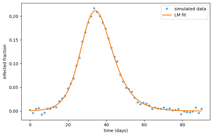
As another example we use SciPy’s LM implementation, available through scipy.optimize.least_squares with method="lm", to fit simulated data from an SEIR model.
The SEIR model describes the spread of an infectious disease through a population by dividing that population into four compartments: susceptible \(S\), exposed \(E\), infected \(I\), and recovered \(R\). Susceptible individuals become exposed on contact with infected individuals, exposed individuals are infected but not yet infectious, and infected individuals eventually recover. Given a set of initial conditions and model parameters, the SEIR model evolves these populations forward in time according to
where the compartments are written as fractions of the total population so that \(S + E + I + R = 1\). The parameter \(\beta\) is the transmission rate, which sets how quickly susceptible individuals become exposed, \(\sigma\) is the rate at which exposed individuals become infectious and is the reciprocal of the mean incubation period, and \(\gamma\) is the recovery rate and is the reciprocal of the mean infectious period. The basic reproduction number follows as \(R_0 = \beta/\gamma\).
Unlike the exponential decay example, this model has no closed form. Each evaluation of \(f(\boldsymbol{\theta}, t)\) requires integrating the system above, so every residual evaluation inside the optimizer costs an ODE solve.
To simulate data we choose \(\boldsymbol{\theta}_\mathrm{true} = \{\beta, \sigma, \gamma\} = \{0.6, 0.5, 0.2\}\), corresponding to a two-day incubation period, a five-day infectious period, and \(R_0 = 3\).
We take initial conditions \(I(0) = 10^{-3}\) with the remainder of the population susceptible, integrate with solve_ivp over ninety days, sample the infected fraction \(I(t)\) at sixty points, and add Gaussian noise of standard deviation \(0.005\).
The fit then treats the initial conditions as known and recovers only the three rate parameters from the noisy \(I(t)\) data.
Note, if you would like further material on solving differentials equations in Python, volume 4, chapters 2 and 3 of the Foundations of Applied Mathematics has relevant information.
import numpy as np
import matplotlib.pyplot as plt
from scipy.integrate import solve_ivp
from scipy.optimize import least_squares

# =====================================================================
# 1. SEIR MODEL
# =====================================================================


def seir_rhs(t, u, beta, sigma, gamma):
    """Right-hand side of the SEIR system"""
    S, E, I, R = u
    dS = -beta * S * I
    dE = beta * S * I - sigma * E
    dI = sigma * E - gamma * I
    dR = gamma * I
    return [dS, dE, dI, dR]


def solve_seir(theta, t_eval, u0):
    """Integrate the SEIR system and return all four compartments"""
    sol = solve_ivp(
        seir_rhs,
        (t_eval[0], t_eval[-1]),
        u0,
        args=tuple(theta),
        t_eval=t_eval,
        rtol=1e-10,
        atol=1e-12,
    )
    return sol.y


# =====================================================================
# 2. SIMULATE NOISY DATA
# =====================================================================

theta_true = np.array([0.6, 0.5, 0.2])  # beta, sigma, gamma

I0 = 1e-3
u0 = [1.0 - I0, 0.0, I0, 0.0]

t_data = np.linspace(0, 90, 60)
I_clean = solve_seir(theta_true, t_data, u0)[2]

rng = np.random.default_rng(42)
I_noisy = I_clean + rng.normal(0, 0.005, size=t_data.shape)

# =====================================================================
# 3. FIT WITH SCIPY'S LEVENBERG-MARQUARDT
# =====================================================================


def residuals(theta, t, I_obs, u0):
    """Residual vector passed to least_squares, one entry per observation"""
    return solve_seir(theta, t, u0)[2] - I_obs


theta_init = np.array([1.0, 1.0, 0.5])

result = least_squares(
    residuals,
    theta_init,
    method="lm",
    args=(t_data, I_noisy, u0),
)

theta_fit = result.x

# Parameter uncertainties from the Gauss-Newton Hessian approximation
dof = len(t_data) - len(theta_fit)
cov = (2 * result.cost / dof) * np.linalg.inv(result.jac.T @ result.jac)
err = np.sqrt(np.diag(cov))

print(f"{'Parameter':<10} | {'True':<8} | {'Fit':<8} | {'Uncertainty':<10}")
print("-" * 46)
for name, tv, fv, ev in zip(["beta", "sigma", "gamma"], theta_true, theta_fit, err):
    print(f"{name:<10} | {tv:<8.3f} | {fv:<8.3f} | {ev:<10.3f}")

print(f"\nFinal cost 0.5 * sum(r^2): {result.cost:.6e}")
print(f"Function evaluations: {result.nfev}")

# =====================================================================
# 4. PLOT
# =====================================================================

t_fine = np.linspace(0, 90, 400)
u_fit = solve_seir(theta_fit, t_fine, u0)

fig, ax = plt.subplots(figsize=(8, 5))
ax.plot(t_data, I_noisy, "o", ms=4, alpha=0.6, label="simulated data")
ax.plot(t_fine, u_fit[2], "-", lw=2, label="LM fit")
ax.set_xlabel("time (days)")
ax.set_ylabel("infected fraction")
ax.legend()
plt.show()
Parameter  | True     | Fit      | Uncertainty
----------------------------------------------
beta       | 0.600    | 0.578    | 0.033
sigma      | 0.500    | 0.549    | 0.088
gamma      | 0.200    | 0.197    | 0.003

Final cost 0.5 * sum(r^2): 4.470063e-04
Function evaluations: 59