4.5. Complex Numbers#
These notes are a work in progress. If you spot any errors or have suggestions, please let us know—your feedback is valuable to us.
In these notes, we cover some basic ideas of complex numbers.
Imaginary numbers, or complex numbers, contain the imaginary unit \(i=\sqrt{-1}\). Consider the algebraic equation
This equation has the explicit solutions
which follow directly from the property that \(i^2 = -1\). In this regard, we see that imaginary numbers are a natural consequence of well-defined algebraic equations. The point is that imaginary numbers are not actually “imaginary” in the colloquial sense; they are a real, rigorous, and highly useful mathematical concept.
The imaginary unit \(i\) in Python is unfortunately denoted by 1j. This notation is a carryover from engineering traditions, where it is standard to use \(j\) for \(\sqrt{-1}\) because the variable \(i\) is conventionally reserved for electrical current. The Python code below demonstrates how to instantiate and square this complex number.
# Defining the imaginary unit in Python
imaginary_i = 1j

# Verifying that i^2 = -1
result = imaginary_i**2
print(f"The square of 1j is: {result}")
from IPython.display import Math, display
import numpy as np
import matplotlib.pyplot as plt

complex_i = 1j

for i in range(5):
    # Wrap the string in Math() to tell Jupyter to render it as LaTeX
    label = Math(fr"i^{{{i}}} = ")
    display(label, complex_i**i)
(1+0j)
1j
(-1+0j)
(-0-1j)
(1+0j)
In Python, complex numbers are represented by the complex type, while NumPy provides specific bit-width types such as complex64 (consisting of two 32-bit floats for the real and imaginary parts) and complex128. If a NumPy array is intended to store complex values, it should be explicitly initialized with a complex data type to prevent the fractional or imaginary components from being truncated. The Python code below demonstrates how to properly initialize a complex NumPy array.
import numpy as np

# Initializing a NumPy array with a complex data type
complex_array = np.array([1 + 2j, 3 + 4j], dtype=np.complex64)

print("Array:", complex_array)
print("Data Type:", complex_array.dtype)
Below is another example.
complex_i = 1j

array = np.zeros(5, dtype="complex64")

for i in range(5):

    array[i]= complex_i**2

array
array([-1.+0.j, -1.+0.j, -1.+0.j, -1.+0.j, -1.+0.j], dtype=complex64)
NumPy complex numbers consist of two elements: a real part and an imaginary part. This follows standard mathematical convention. Suppose \(z\) is a complex number with a real component \(a\) and an imaginary component \(b\),
Both \(a\) and \(b\) are real numbers, where
and
The following Python code defines a complex number and extracts its real and imaginary components.
# Define a complex number
z = 5 - 2j

# Extract real and imaginary parts
real_part = np.real(z)
imag_part = np.imag(z)

print(f"Real part: {real_part}")
print(f"Imaginary part: {imag_part}")
Real part: 5.0
Imaginary part: -2.0
The complex conjugate of a complex number \(z\) is denoted as \(z^*\) and is formed by changing the sign of the imaginary part. For \(z = a + ib\), the complex conjugate is
The following Python code demonstrates how to find the complex conjugate using NumPy.
# Define a complex number
z = 3 + 4j

# Calculate the complex conjugate
z_conjugate = np.conj(z)

print(f"Original: {z}")
print(f"Conjugate: {z_conjugate}")
Original: (3+4j)
Conjugate: (3-4j)
4.5.1. Argand Diagram and Polar Form#
An Argand diagram represents a complex number as a point or vector in a two-dimensional space called the complex plane. The real part is plotted along the horizontal axis, and the imaginary part is plotted along the vertical axis, mirroring how Cartesian coordinates map a two-dimensional vector.
The distance from the origin to the complex number is its magnitude. This distance can be computed geometrically using the Pythagorean theorem,
Alternatively, the magnitude can be calculated using the complex conjugate,
The following Python code plots a complex number on the complex plane and demonstrates three equivalent ways to calculate its magnitude using NumPy: via the Pythagorean theorem, the complex conjugate, and the linear algebra package.
# Define complex number
z = 3 + 4j
a = np.real(z)
b = np.imag(z)

# 1. Magnitude via Pythagorean theorem
mag_pythag = np.sqrt(a**2 + b**2)

# 2. Magnitude via complex conjugate
mag_conj = np.sqrt(z * np.conj(z)).real

# 3. Magnitude via NumPy's linalg package
mag_linalg = np.linalg.norm([a, b])

print("--- Magnitude Calculations ---")
print(f"Pythagorean Theorem: {mag_pythag:.4f}")
print(f"Complex Conjugate:   {mag_conj:.4f}")
print(f"NumPy Linalg Norm:   {mag_linalg:.4f}\n")
--- Magnitude Calculations ---
Pythagorean Theorem: 5.0000
Complex Conjugate:   5.0000
NumPy Linalg Norm:   5.0000
# Define complex number
z = 3 + 4j
a = np.real(z)
b = np.imag(z)

# Plotting the complex number on an Argand diagram
plt.figure(figsize=(6, 6))
plt.axhline(0, color='black', linewidth=0.8)
plt.axvline(0, color='black', linewidth=0.8)

# Plot the vector and the point
plt.quiver(0, 0, a, b, angles='xy', scale_units='xy', scale=1, color='blue', zorder=3)
plt.scatter(a, b, color='red', zorder=5)

# Annotate the explicit point z
plt.text(a + 0.1, b + 0.1, f'$z = {int(a)} + {int(b)}j$', fontsize=12, weight='bold')

# Add adjacent (real) and opposite (imaginary) sides to form a right triangle
plt.plot([0, a], [0, 0], color='purple', linestyle='--', linewidth=1.5, label='Real component (a)')
plt.plot([a, a], [0, b], color='green', linestyle='--', linewidth=1.5, label='Imaginary component (b)')

# Label the adjacent and opposite sides directly on the plot
plt.text(a / 2, -0.3, f'a = {int(a)}', color='purple', fontsize=10, ha='center')
plt.text(a + 0.1, b / 2, f'b = {int(b)}', color='green', fontsize=10, va='center')

# Axis limits and labels (using raw strings 'r' to prevent SyntaxWarnings)
plt.xlim(-1, 5)
plt.ylim(-1, 5)
plt.xlabel(r'Real Axis ($\mathcal{Re}$)')
plt.ylabel(r'Imaginary Axis ($\mathcal{Im}$)')
plt.title('Argand Diagram with Geometric Components')
plt.grid(True, linestyle=':', alpha=0.6)
plt.legend(loc='upper left')
<matplotlib.legend.Legend at 0x10d76aa50>
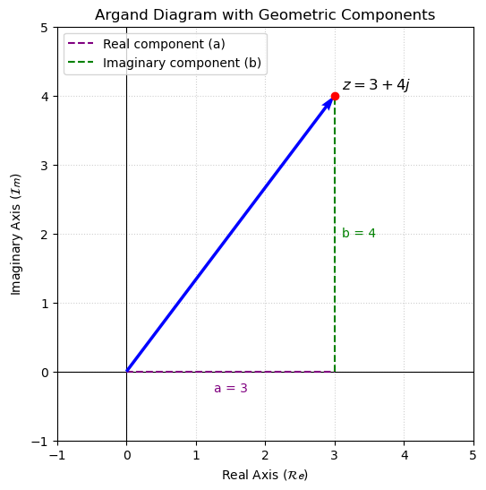
We can also express a complex number in polar form. Let \(r\) be the magnitude of the complex number, \(r = |z|\). From the geometry of the Argand diagram, the real part is \(\mathcal{Re}(z) = r \cos \theta\) and the imaginary part is \(\mathcal{Im}(z) = r\sin \theta\), where the angle \(\theta\) is given by
Substituting these into the Cartesian form yields the polar representation
Using Euler’s formula, \(e^{i\theta} = \cos \theta + i \sin \theta\), this simplifies compactly to
Because the trigonometric functions \(\cos \theta\) and \(\sin \theta\) are periodic with a period of \(2\pi\), adding any integer multiple of \(2\pi\) to the angle describes the exact same complex number. Consequently, the polar form can be written more generally as
where \(n\) is any integer (\(n = 0, \pm 1, \pm 2, \dots\)). The angle \(\theta\) is called the argument of \(z\), and the unique value of \(\theta\) that falls within the interval \((-\pi, \pi]\) is referred to as the principal argument.
The following Python code demonstrates this equivalence by comparing a complex number generated with a base angle \(\theta\) to one generated with an added phase of \(2n\pi\). As shown by the outputs, both approaches yield identical real and imaginary components.
# Define magnitude and base angle (30 degrees in radians)
r = 10
theta_base = np.radians(30)

# Calculate z with the base angle
z_base = r * np.exp(1j * theta_base)

print("--- Base Angle (theta) ---")
print(f"Real part:      {np.real(z_base):.4f}")
print(f"Imaginary part: {np.imag(z_base):.4f}")

# Add 2*n*pi to the angle
n = 5
theta_shifted = theta_base + n * 2 * np.pi

# Calculate z with the shifted angle
z_shifted = r * np.exp(1j * theta_shifted)

print(f"\n--- Shifted Angle (theta + {n}*2*pi) ---")
print(f"Real part:      {np.real(z_shifted):.4f}")
print(f"Imaginary part: {np.imag(z_shifted):.4f}")
--- Base Angle (theta) ---
Real part:      8.6603
Imaginary part: 5.0000

--- Shifted Angle (theta + 5*2*pi) ---
Real part:      8.6603
Imaginary part: 5.0000