8.1. Feed Forward Neural Networks#
8.1.1. Introduction to Neural Networks#
In these notes, we explore the fundamentals of a basic artificial neural network. Initially, we will focus on the classification of handwritten digits, using the MNIST dataset for multi-class digit recognition and the Breast Cancer Wisconsin dataset for binary classification. The MNIST database consists of \(60{,}000\) training images and a further \(10{,}000\) test images of handwritten digits ranging from 0 through 9, each a \(28 \times 28\) grayscale image. The breast cancer dataset contains 569 instances described by 30 continuous features, which are used to predict whether a tumor is benign or malignant.
8.1.1.1. References#
Neural networks are a supervised learning method, meaning they are trained on data for which the correct answers are known. A neural network models the mapping between predictive features \(\mathbf{X}\) and target variables \(\mathbf{y}\), and I find it useful to view the network as nothing more than a non-linear mapping between these two. The structure is a chain of linear transformations of the data, each followed by a non-linear activation function. The linear transformations alone would compose into a single linear transformation no matter how many were chained together, so it is the activation function that makes the network a genuinely non-linear mapping. The parameters of the network are the weights \(W\) and biases \(\mathbf{b}\) of each linear transformation, and these are what training adjusts.
For a network of \(L\) layers the mapping proceeds as
where \(f\) is the non-linear activation function applied at every hidden layer and \(\mathbf{a}^{(L)}\) is the output of the network. Each layer takes the activations of the layer before it as input, so the data are transformed repeatedly as they pass forward through the network, which is why this is called a feed-forward network. The superscripts index the layer, and each layer carries its own weight matrix and bias vector.
The activation applied at the output layer, written \(g\) above, is generally not the same function used in the hidden layers, and is instead chosen to match the task. For the multi-class MNIST problem we use the softmax function, which converts the output scores into non-negative values summing to one that can be read as class probabilities. For the binary breast cancer problem a single sigmoid output suffices, giving the probability that the tumor is malignant. For a regression problem the output layer would carry no activation at all.
A neural network consists of layers of interconnected processing units called neurons. The leftmost column represents the input layer, where the number of units corresponds directly to the number of features in the dataset. The rightmost column is the output layer, whose dimension matches the number of target classes. Intermediate layers between the input and output layers are referred to as hidden layers, so named because their values are never observed directly in the data and exist only as intermediate representations constructed by the network.

Every neuron in a given layer receives input from all neurons in the preceding layer, as indicated by the arrows in the diagram above, which is why this architecture is called fully connected. The total signal received by a neuron is a linear combination of the outputs from the previous layer plus a scalar offset called the bias. For instance, the net input signal to the top neuron in the hidden layer of the diagram is
where \(a_1, a_2, a_3\) are the outputs of the three input-layer units, the weights \(W_{1j}\) and the bias \(b_1\) are real-valued parameters, and the first index of \(W_{1j}\) identifies the receiving neuron while the second identifies the sending one. The neuron then applies the activation function to produce its own output \(a_1^{(2)} = f(z_1)\), which is passed on to the next layer.
Collecting the analogous expressions for every neuron in the layer recovers the matrix form \(\mathbf{z} = W\mathbf{a} + \mathbf{b}\) from the previous section, where each row of \(W\) holds the weights belonging to one receiving neuron. The weights control how strongly each incoming signal contributes, and the bias shifts the neuron’s threshold for activation, allowing it to respond even when all its inputs are zero.
Counting the parameters makes the scale of the problem concrete. A layer with \(n_{\text{in}}\) inputs and \(n_{\text{out}}\) neurons has \(n_{\text{in}} \times n_{\text{out}}\) weights and \(n_{\text{out}}\) biases.
8.1.2. Problem#
Consider a small toy network in which the input is \(\mathbf{X} \in \mathbb{R}^{3}\) and the target is \(\mathbf{y} \in \mathbb{R}^{2}\), with two hidden layers containing 10 and 5 neurons respectively. Using the convention \(\mathbf{z}^{(\ell)} = W^{(\ell)} \mathbf{a}^{(\ell-1)} + \mathbf{b}^{(\ell)}\), determine the shape of the weight matrix and bias vector for every layer, and find the total number of trainable parameters in the network.
Solution
The network is specified by the layer list \([3, 10, 5, 2]\), which gives three weight matrices, one for each transition between consecutive layers. Note that a list of four numbers produces three sets of parameters, not four, since the input layer holds the data and carries no weights of its own.
The shape of each weight matrix follows from requiring the matrix-vector product to be defined. The matrix \(W^{(\ell)}\) acts on the activation vector \(\mathbf{a}^{(\ell-1)}\) coming from the previous layer and must produce a vector of length equal to the number of neurons in layer \(\ell\), so \(W^{(\ell)}\) has shape \((n_\ell, n_{\ell-1})\), with the receiving layer giving the number of rows and the sending layer the number of columns. The bias vector \(\mathbf{b}^{(\ell)}\) is added to the result, so it has one entry per neuron in layer \(\ell\).
Layer 1 maps the 3-dimensional input to the first hidden layer of 10 neurons, so
giving \(10 \times 3 = 30\) weights and 10 biases, for 40 parameters.
Layer 2 maps the first hidden layer of 10 neurons to the second hidden layer of 5 neurons, so
giving \(5 \times 10 = 50\) weights and 5 biases, for 55 parameters.
Layer 3 maps the second hidden layer of 5 neurons to the 2-dimensional output, so
giving \(2 \times 5 = 10\) weights and 2 biases, for 12 parameters.
Summing over the three layers, the network has \(30 + 50 + 10 = 90\) weights and \(10 + 5 + 2 = 17\) biases, for a total of
In general, for a network specified by the layer list \([n_0, n_1, \ldots, n_L]\) the total parameter count is
where the first term counts the weights and the second the biases. Notice that the biases are a small fraction of the total, 17 out of 107 here, and that the fraction shrinks as layers grow wider, since the weight count grows as the product of two layer sizes while the bias count grows only as one.
The following code confirms the count.
import numpy as np

layers = [3, 10, 5, 2]

total = 0
for i in range(len(layers) - 1):
    n_in, n_out = layers[i], layers[i+1]
    n_w, n_b = n_out * n_in, n_out
    print(f"Layer {i+1}: W shape ({n_out}, {n_in}), b shape ({n_out},), "
          f"{n_w} weights + {n_b} biases = {n_w + n_b}")
    total += n_w + n_b

print(f"Total parameters: {total}")
A common mistake is to write \(W^{(1)}\) as a \(3 \times 10\) matrix by reading the layer sizes left to right. That ordering is not wrong in itself, but it corresponds to the alternative convention \(\mathbf{z} = \mathbf{a} W + \mathbf{b}\) with row vectors, which is what NumPy broadcasting favors when data are stored with one sample per row. Either convention works as long as it is applied consistently throughout the network; mixing the two is the single most common source of shape errors when implementing a network from scratch.
8.1.2.1. Mathematical Conventions#
Throughout these notes, we adhere to the following notation and indexing conventions.
Bold lowercase symbols denote vectors and uppercase symbols denote matrices, so \(\mathbf{a}\) is an activation vector and \(W\) a weight matrix
\(i\) indexes individual training or testing examples
\(\ell\) denotes the network layer, where \(\ell = 0\) is the input layer and \(\ell = L\) is the output layer, so a network with \(L\) layers has \(L\) weight matrices and \(L\) bias vectors
Superscripts in parentheses identify the layer and subscripts identify the neuron, so \(a_j^{(\ell)}\) is the activation of neuron \(j\) in layer \(\ell\)
\(j, k\) index individual neurons within a given layer, with \(j\) referring to the receiving layer and \(k\) to the sending layer, so \(W_{jk}^{(\ell)}\) is the weight connecting neuron \(k\) in layer \(\ell-1\) to neuron \(j\) in layer \(\ell\)
\(n_\ell\) is the number of neurons in layer \(\ell\), so \(W^{(\ell)}\) has shape \(n_\ell \times n_{\ell-1}\)
\(f\) denotes the activation function applied at the hidden layers and \(g\) the activation applied at the output layer
Partial derivatives are abbreviated as \(\partial f / \partial x = \partial_x f\)
8.1.2.2. Activations#
To introduce non-linearity and enable learning of complex decision boundaries, an activation function is applied elementwise to the linear combination \(z^{(\ell)}_j = W^{(\ell)}_{jk} a^{(\ell-1)}_k + b^{(\ell)}_j\). Activation functions serve several theoretical and practical roles.
Expressive Power: Without a non-linear activation function, a multi-layer network collapses mathematically into a single composite linear transformation, rendering the hidden layers redundant. This is the essential reason the activation is there at all.
Smoothness and Differentiability: Classification targets are discrete step functions, mapping class labels to 0 or 1. A step function has zero derivative almost everywhere, which makes gradient-based optimization impossible. Activation functions provide a smooth surrogate with well-defined derivatives throughout the network.
Input-Dependent Gradients: Applying non-linear transformations ensures that the gradient of the loss retains dependence on the input values, enabling parameter updates that respond to the local structure of the data.
The activation applied at layer \(\ell\) produces the output vector
which is passed forward as input to the next layer. This forward propagation step continues layer by layer through the output layer \(\ell = L\).
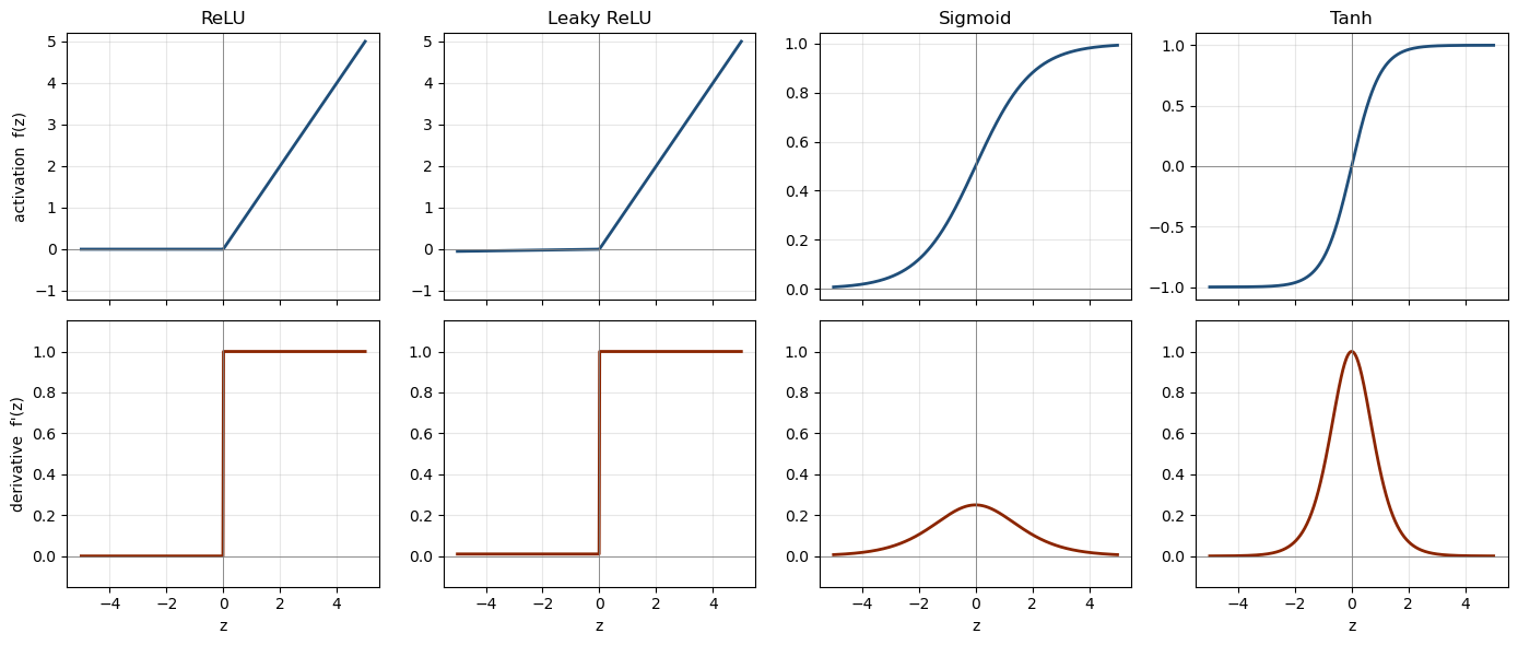
Since training requires the derivative of the activation at every layer, we list each function together with its derivative.
ReLU is the default choice for hidden layers in modern networks and should be your first choice unless you have a specific reason otherwise. It is defined as
and is undefined at \(z = 0\), where implementations conventionally take \(f'(0) = 0\). Its derivative is exactly 1 for positive inputs, so gradients pass through activated units undiminished, which is what allows deep networks to train. It is also trivially cheap to evaluate. The drawback is that units with negative pre-activation pass exactly zero gradient, and a unit driven permanently negative stops learning entirely.
Leaky ReLU addresses that failure by allowing a small negative slope \(\alpha\), typically \(0.01\),
so that no unit can ever receive exactly zero gradient.
The logistic sigmoid maps the real line to \((0,1)\) and is written
The derivative is worth committing to memory, since expressing it in terms of the function value means the forward pass output can be reused in the backward pass. Its maximum value is \(\sigma'(0) = 1/4\), so every sigmoid layer shrinks the gradient by at least a factor of four during backpropagation, and far more when units are saturated. This is the vanishing gradient problem, and it is the reason sigmoid is no longer used in hidden layers. It remains the correct choice for a single output unit in binary classification, where the output must be a probability.
The hyperbolic tangent is a rescaled sigmoid mapping to \((-1, 1)\),
Its derivative reaches 1 at the origin rather than \(1/4\), and its output is centered at zero, both of which make it preferable to the sigmoid. It saturates just as badly for large \(|z|\), however, so it suffers the same vanishing gradient problem in deep networks.
The code below plots each activation function together with its derivative.
Comparing the bottom row of the resulting figure makes the case for ReLU immediately. The ReLU derivative is a flat line at 1 over the entire positive half-axis, while the sigmoid and tanh derivatives are narrow bumps that fall to zero within a few units of the origin. A neuron whose pre-activation drifts outside that narrow window receives essentially no gradient, and the deeper the network the more likely that becomes.
import numpy as np
import matplotlib.pyplot as plt

def relu(z):            return np.maximum(0.0, z)
def d_relu(z):          return np.where(z > 0, 1.0, 0.0)

def leaky(z, a=0.01):   return np.where(z > 0, z, a*z)
def d_leaky(z, a=0.01): return np.where(z > 0, 1.0, a)

def sigmoid(z):         return 1.0/(1.0 + np.exp(-z))
def d_sigmoid(z):       s = sigmoid(z); return s*(1.0 - s)

def tanh(z):            return np.tanh(z)
def d_tanh(z):          return 1.0 - np.tanh(z)**2

z = np.linspace(-5, 5, 500)
funcs = [("ReLU", relu, d_relu),
         ("Leaky ReLU", leaky, d_leaky),
         ("Sigmoid", sigmoid, d_sigmoid),
         ("Tanh", tanh, d_tanh)]

fig, axes = plt.subplots(2, 4, figsize=(14, 6), sharex=True)

for col, (name, f, df) in enumerate(funcs):
    axes[0, col].plot(z, f(z), lw=2, color="#1f4e79")
    axes[0, col].set_title(name)
    axes[1, col].plot(z, df(z), lw=2, color="#8b2500")
    for row in (0, 1):
        axes[row, col].axhline(0, color="gray", lw=0.6)
        axes[row, col].axvline(0, color="gray", lw=0.6)
        axes[row, col].grid(alpha=0.3)
    axes[1, col].set_xlabel("z")
    axes[1, col].set_ylim(-0.15, 1.15)

axes[0, 0].set_ylabel("activation  f(z)")
axes[1, 0].set_ylabel("derivative  f'(z)")
axes[0, 0].set_ylim(-1.2, 5.2)
axes[0, 1].set_ylim(-1.2, 5.2)

plt.tight_layout()
8.1.3. Training the Network#
The weights and biases are initialized randomly, and the exact details of the initialization will be addressed later. The goal of training is to determine the values of the weights and biases so that the model best fits the data. Once again, we need a loss function to measure the degree of fit, and the appropriate choice depends on the task.
For regression problems, in which the target is a continuous value, the mean squared error is the common choice,
where \(N\) is the number of training examples, \(y_i\) is the target value for example \(i\), and \(\hat{y}_i\) is the network prediction.
For classification problems, we use the categorical cross entropy,
where \(C\) is the number of classes, \(y_{ic}\) is the one-hot encoded label taking the value 1 when example \(i\) belongs to class \(c\) and 0 otherwise, and \(\hat{y}_{ic}\) is the probability the network assigns to class \(c\) for example \(i\). Because the one-hot label is zero for every class except the correct one, the inner sum collapses to a single term, and the loss for one example reduces to \(-\log \hat{y}_{ic^*}\) where \(c^*\) is the true class. The loss therefore depends only on the probability the network assigned to the correct answer, growing without bound as that probability approaches zero.
When the classification is binary, with only two classes, the categorical cross entropy reduces to the log loss,
where \(y_i \in \{0, 1\}\) and \(\hat{y}_i\) is the single sigmoid output giving the probability that example \(i\) belongs to class 1. Only one of the two terms in the bracket is active for any given example, depending on whether the label is 0 or 1.
Note that mean squared error should not be used for classification even though it is possible to do so. Paired with a softmax or sigmoid output, the squared error produces vanishingly small gradients when the network is confidently wrong, which is exactly when large gradients are needed. The cross entropy does not have this defect.
Having chosen a loss function, we minimize it with respect to the parameters. To start with, we will optimize with batch gradient descent, in which we construct the gradient over all training data before taking a step. Collecting every weight and bias in the network into a single parameter vector \(\boldsymbol{\theta}\) (i.e., \(\theta=\{\mathbf{W},~ \mathbf{b}\})\), the update is
where \(\eta\) is the learning rate and the gradient is
with \(L_i\) the loss contributed by training example \(i\). Written out for an individual parameter, the same update reads
The gradient points in the direction of steepest increase of the loss, so stepping opposite to it decreases the loss for a sufficiently small learning rate. Every parameter in the network is updated simultaneously using the gradient evaluated at the current parameter values.
Batch gradient descent requires a full pass over the training data for every single update, which is why it is impractical for large datasets and why we will replace it with mini-batch gradient descent shortly. The remaining difficulty is computing \(\partial L / \partial W^{(\ell)}_{jk}\) for parameters buried deep in the network, where the loss depends on the parameter only through a long chain of subsequent layers. This is what backpropagation solves.
8.1.3.1. Backpropagation#
Backpropagation is the efficient way to compute the gradient of the loss with respect to every weight and bias. The gradients are computed with the chain rule, but the chain rule alone is not the point. The point is bookkeeping: a naive application of the chain rule recomputes the same quantities over and over, once for every parameter, while backpropagation computes each shared quantity a single time and passes it backward through the network.
The quantity worth tracking is the derivative of the loss with respect to the pre-activation of a layer,
which we will call the error at layer \(\ell\). Everything in this section follows from the observation that once \(\boldsymbol{\delta}^{(\ell)}\) is known, both the weight and bias gradients at that layer follow immediately, and \(\boldsymbol{\delta}^{(\ell-1)}\) can be obtained from it.
8.1.3.1.1. The last layer#
Consider the output layer \(\ell = L\), where \(\mathbf{z}^{(L)} = W^{(L)} \mathbf{a}^{(L-1)} + \mathbf{b}^{(L)}\) and the loss is some function of the network output. Applying the chain rule to an individual weight gives
where the second factor follows because \(z^{(L)}_j = \sum_k W^{(L)}_{jk} a^{(L-1)}_k + b^{(L)}_j\) depends on \(W^{(L)}_{jk}\) only through the single term \(W^{(L)}_{jk} a^{(L-1)}_k\). Similarly, since \(\partial z^{(L)}_j / \partial b^{(L)}_j = 1\),
In matrix form these read
The weight gradient is an outer product of the error at the layer with the activations feeding into it, which is worth noticing because the same structure appears at every layer.
For a general loss and output activation \(g\), the error at the output layer is
where \(\odot\) denotes elementwise multiplication. For the specific case of a softmax output paired with categorical cross entropy, this simplifies dramatically to
the predicted probability vector minus the one-hot label. This is the reason for pairing softmax with cross entropy rather than differentiating the two separately.
8.1.3.1.2. The second to last layer#
Now consider layer \(L-1\). Its pre-activation \(\mathbf{z}^{(L-1)}\) influences the loss only through \(\mathbf{a}^{(L-1)} = f(\mathbf{z}^{(L-1)})\), which in turn feeds every neuron of the output layer. Because \(a^{(L-1)}_k\) appears in all of the \(z^{(L)}_j\), the chain rule requires a sum over \(j\),
which is the matrix-vector product \(\left(W^{(L)}\right)^T \boldsymbol{\delta}^{(L)}\). Passing through the activation function then gives the error at layer \(L-1\),
This is the essential step. The error at layer \(L-1\) is obtained from the error at layer \(L\) by multiplying by the transpose of the weight matrix and by the derivative of the activation. Nothing from the forward pass beyond \(\mathbf{z}^{(L-1)}\) is needed, and no derivative is recomputed.
With \(\boldsymbol{\delta}^{(L-1)}\) in hand, the gradients follow by exactly the same argument as before,
8.1.3.1.3. The general layer#
Nothing in the previous step was specific to layer \(L-1\). The same relation holds between any two adjacent layers, so the error propagates backward through the network according to
and at every layer the parameter gradients are
with \(\mathbf{a}^{(0)} = \mathbf{X}\) the input data at the first layer.
The complete algorithm is therefore a forward pass storing every \(\mathbf{z}^{(\ell)}\) and \(\mathbf{a}^{(\ell)}\), followed by a backward pass starting from \(\boldsymbol{\delta}^{(L)}\) and applying the recursion above until layer 1 is reached, accumulating the parameter gradients along the way. The cost of the backward pass is comparable to the forward pass, so the full gradient with respect to all \(\dim(\boldsymbol{\theta})\) parameters costs roughly twice a single evaluation of the network. This is what makes training feasible: computing 89,610 partial derivatives by finite differences would require 89,610 separate forward passes.
The storage requirement is the price paid. Every activation from the forward pass must be kept until the backward pass consumes it, which is why memory scales with network depth and batch size.
8.1.3.1.4. Why the vanishing gradient problem appears here#
The recursion makes the vanishing gradient problem explicit. Unrolling it from the output back to layer \(\ell\) shows that \(\boldsymbol{\delta}^{(\ell)}\) carries one factor of \(f'\) for every layer the error has passed through. If those factors are typically smaller than one, as they are for the sigmoid where \(f' \le 1/4\), the product decays geometrically with depth and the early layers receive almost no gradient. For ReLU the factor is exactly 1 wherever a unit is active, so no such decay occurs.
8.1.4. Example: Breast Cancer Dataset#
Let us put this all together in an example, coding a neural network from scratch using the Breast Cancer Wisconsin dataset. We will use ReLU activations in the hidden layers, a single sigmoid output unit, and the binary log loss, with a network of two hidden layers.
8.1.4.1. Loading and preparing the data#
The dataset contains 569 instances, each described by 30 continuous features computed from a digitized image of a fine needle aspirate of a breast mass. The features describe properties of the cell nuclei present in the image, such as radius, texture, perimeter, area, and smoothness, with the mean, standard error, and worst value recorded for each of ten base measurements. The target is binary: 212 of the instances are malignant and 357 are benign. Note that in the scikit-learn version of the dataset the label 0 corresponds to malignant and 1 to benign, which is worth checking before interpreting any result.
The architecture follows from the data. The input layer must have 30 units, one per feature, and the output layer has a single unit whose sigmoid activation gives the probability that the tumor is benign. We choose two hidden layers of 16 and 8 neurons, giving the layer list \([30, 16, 8, 1]\).
We pass stratify=y so that the class proportions are preserved in both splits, which matters here because the classes are unbalanced roughly 63/37.
8.1.4.2. Training#
We train with full-batch gradient descent, computing the gradient over all training examples before each update. The training set here has only 455 examples, so a full-batch gradient is cheap; for MNIST we will need mini-batches.
def train(X, y, X_val, y_val, layers, eta=0.1, epochs=2000, seed=0):
    W, b = initialize(layers, seed)
    history = {"train": [], "val": []}

    for epoch in range(epochs):
        Z, A = forward(X, W, b)
        dW, db = backward(y, Z, A, W)

        for l in range(len(W)):
            W[l] -= eta * dW[l]
            b[l] -= eta * db[l]

        history["train"].append(log_loss(y, A[-1]))
        history["val"].append(log_loss(y_val, forward(X_val, W, b)[1][-1]))

    return W, b, history

layers = [30, 16, 8, 1]
W, b, history = train(X_train, y_train, X_test, y_test, layers, eta=0.1, epochs=2000)
8.1.4.3. Evaluating#
A sigmoid output gives a probability, so a threshold is needed to produce a class label. The default choice of 0.5 is reasonable when the classes are roughly balanced.
def predict(X, W, b, threshold=0.5):
    return (forward(X, W, b)[1][-1] >= threshold).astype(int)

train_acc = np.mean(predict(X_train, W, b) == y_train)
test_acc = np.mean(predict(X_test, W, b) == y_test)

print(f"training accuracy: {train_acc:.4f}")
print(f"test accuracy:     {test_acc:.4f}")
Plotting the two loss curves together shows whether the network is generalizing or memorizing.
import matplotlib.pyplot as plt

fig, ax = plt.subplots(figsize=(7, 4.5))
ax.plot(history["train"], lw=2, label="training loss")
ax.plot(history["val"], lw=2, label="test loss")
ax.set_xlabel("epoch")
ax.set_ylabel("binary log loss")
ax.legend()
ax.grid(alpha=0.3)
plt.show()
A network of this size on a dataset of this size will reach high accuracy, well above 95%, and the training loss will continue to fall after the test loss has flattened or begun to rise. That gap is overfitting, and with 30 features, 569 examples, and a network carrying several hundred parameters it is entirely expected.
8.1.4.4. Things worth trying#
Confirm that standardization matters by rerunning with the raw features and watching the training fail or crawl.
Confirm that accuracy alone is a misleading metric here. Because 63% of the instances are benign, a model that predicts benign for every input achieves 63% accuracy while being clinically useless. Compute the confusion matrix instead, and note that a false negative, a malignant tumor classified as benign, is a far more serious error than a false positive. Lowering the decision threshold below 0.5 trades precision for recall and may be the right choice for this application.
Finally, vary the architecture. Try a single hidden layer, try wider layers, and see how little difference it makes on a problem this small and nearly linearly separable.
from sklearn.datasets import load_breast_cancer
from sklearn.model_selection import train_test_split

data = load_breast_cancer()
X, y = data.data, data.target.reshape(-1, 1)

print("feature matrix shape:", X.shape)
print("target shape:        ", y.shape)
print("class balance:       ", np.bincount(y.ravel()))

X_train, X_test, y_train, y_test = train_test_split(
    X, y, test_size=0.2, random_state=42, stratify=y
)

print("training samples:", X_train.shape[0])
print("test samples:    ", X_test.shape[0])
feature matrix shape: (569, 30)
target shape:         (569, 1)
class balance:        [212 357]
training samples: 455
test samples:     114
The features in this dataset live on different scales. Mean area runs into the hundreds while mean smoothness is a number around 0.1, a difference of three orders of magnitude. Feeding raw features into a network is a poor idea, since a weight update of a given size has an enormous effect on the small-scale features and a negligible one on the large-scale features, producing exactly the badly conditioned optimization landscape that makes gradient descent zigzag.
We therefore standardize each feature to zero mean and unit variance,
where \(\mu_j\) and \(\sigma_j\) are the mean and standard deviation of feature \(j\).
The critical detail is that \(\mu\) and \(\sigma\) are computed from the training data only and then applied to the test data. Computing them from the full dataset would leak information about the test set into the training process, and the resulting test accuracy would be optimistic. This is the same principle as centering the test data with the training mean in the PCA anomaly detection exercise.
mu = X_train.mean(axis=0)
sigma = X_train.std(axis=0)

X_train = (X_train - mu) / sigma
X_test = (X_test - mu) / sigma
# check
print(X_train.mean(axis=0)[:5])
print(X_train.std(axis=0)[:5])
print(X_train.min(), X_train.max())
[-4.31742554e-15  2.24606658e-15 -7.38359313e-16  1.71779562e-16
  5.22695440e-15]
[1. 1. 1. 1. 1.]
-2.715107359251433 11.658389001118913
8.1.4.5. Building the network#
The implementation follows the forward and backward passes derived in the previous section. We store the weights and biases in lists indexed by layer, so that the architecture is determined entirely by the layer list passed in.
def forward(X, W, b):
    """Return the pre-activations Z and activations A for every layer."""
    A = [X]
    Z = []
    L = len(W)
    for l in range(L):
        z = np.dot(A[-1], W[l].T) + b[l]
        Z.append(z)
        A.append(relu(z) if l < L - 1 else sigmoid(z))
    return Z, A
def initialize(layers, seed=0):
    """He initialization for weights, zeros for biases."""
    rng = np.random.default_rng(seed)
    W, b = [], []
    for i in range(len(layers) - 1):
        n_in, n_out = layers[i], layers[i+1]
        W.append(rng.normal(0, np.sqrt(2.0 / n_in), size=(n_out, n_in)))
        b.append(np.zeros(n_out))
    return W, b

def relu(z):        return np.maximum(0.0, z)
def d_relu(z):      return (z > 0).astype(float)

def sigmoid(z):
    """safe sigmoid."""
    out = np.empty_like(z, dtype=float)
    pos = z >= 0
    out[pos] = 1.0 / (1.0 + np.exp(-z[pos]))
    ez = np.exp(z[~pos])
    out[~pos] = ez / (1.0 + ez)
    return out
8.1.4.6. Evaluating#
A sigmoid output gives a probability, so a threshold is needed to produce a class label. The default choice of 0.5 is reasonable when the classes are roughly balanced.
Let use evaluate with the random initializations and then check after training.
def predict(X, W, b, threshold=0.5):
    return (forward(X, W, b)[1][-1] >= threshold).astype(int)

W, b = initialize(layers, 42)
train_acc = np.mean(predict(X_train, W, b) == y_train)
test_acc = np.mean(predict(X_test, W, b) == y_test)

print(f"training accuracy: {train_acc:.4f}")
print(f"test accuracy:     {test_acc:.4f}")
---------------------------------------------------------------------------
NameError                                 Traceback (most recent call last)
/var/folders/mq/8_f0y54n1g3f0ht8yb9b6by40000gn/T/ipykernel_79979/3497241526.py in <cell line: 0>()
      2     return (forward(X, W, b)[1][-1] >= threshold).astype(int)
      3
----> 4 W, b = initialize(layers, 42)
      5 train_acc = np.mean(predict(X_train, W, b) == y_train)
      6 test_acc = np.mean(predict(X_test, W, b) == y_test)

NameError: name 'layers' is not defined
The log-loss function is constructed below.
def log_loss(y, yhat, eps=1e-12):
    yhat = np.clip(yhat, eps, 1 - eps)
    return -np.mean(y * np.log(yhat) + (1 - y) * np.log(1 - yhat))
The backward pass starts from the output error and applies the recursion \(\boldsymbol{\delta}^{(\ell)} = \left[ \left(W^{(\ell+1)}\right)^T \boldsymbol{\delta}^{(\ell+1)} \right] \odot f'(\mathbf{z}^{(\ell)})\). For a sigmoid output paired with the log loss, the output error simplifies to \(\hat{y} - y\), exactly as the softmax and cross entropy pairing did.
def backward(y, Z, A, W):
    """Return gradients dW, db for every layer."""
    N = y.shape[0]
    L = len(W)
    dW = [None] * L
    db = [None] * L

    delta = (A[-1] - y) / N          # sigmoid output + log loss

    for l in reversed(range(L)):
        dW[l] = np.dot(delta.T, A[l])
        db[l] = delta.sum(axis=0)
        if l > 0:
            delta = np.dot(delta, W[l]) * d_relu(Z[l-1])

    return dW, db
8.1.4.7. Training#
We train with full-batch gradient descent, computing the gradient over all training examples before each update. The training set here has only 455 examples, so a full-batch gradient is cheap; for MNIST we will need mini-batches.
def train(X, y, X_val, y_val, layers, eta=0.05, epochs=2000, seed=0):
    if np.abs(X.mean()) > 1.0 or not (0.5 < X.std() < 2.0):
        raise ValueError(
            f"Features look unstandardized (mean {X.mean():.3f}, std {X.std():.3f}). "
            "Run the standardization cell before training."
        )

    W, b = initialize(layers, seed)
    history = {"train": [], "val": []}

    for epoch in range(epochs):
        Z, A = forward(X, W, b)
        dW, db = backward(y, Z, A, W)

        if not np.isfinite(dW[0]).all():
            raise FloatingPointError(
                f"Gradient became non-finite at epoch {epoch}. "
                "Lower the learning rate."
            )

        for l in range(len(W)):
            W[l] -= eta * dW[l]
            b[l] -= eta * db[l]

        history["train"].append(log_loss(y, A[-1]))
        history["val"].append(log_loss(y_val, forward(X_val, W, b)[1][-1]))

    return W, b, history

layers = [30, 16, 8, 1]
W, b, history = train(X_train, y_train, X_test, y_test, layers, eta=0.1, epochs=2000)
# Plotting the two loss curves together shows whether the network is generalizing or memorizing.


fig, ax = plt.subplots(figsize=(7, 4.5))
ax.plot(history["train"], lw=2, label="training loss")
ax.plot(history["val"], lw=2, label="test loss")
ax.set_xlabel("epoch")
ax.set_ylabel("binary log loss")
ax.legend()
ax.grid(alpha=0.3)
plt.show()
That looks like we overfitted. We should have stopped training at around 100 epochs. After that predictions for the test data got worse. Let’s check our final accuracy.
train_acc = np.mean(predict(X_train, W, b) == y_train)
test_acc = np.mean(predict(X_test, W, b) == y_test)

print(f"training accuracy: {train_acc:.4f}")
print(f"test accuracy:     {test_acc:.4f}")
8.1.5. Finding the Best Architecture#
How do we determine the best architecture, meaning the number of hidden layers and the number of neurons in each? There is no absolute best way to do this (at least that is what I know).
An approach is to experiment with several candidate architectures and compare them on data the network has not trained on.
The obvious comparison, training each candidate and picking the one with the highest test accuracy, is a trap. Choosing the architecture using the test set means the test set has influenced the model, and the resulting accuracy is no longer an honest estimate of how the network will perform on new data. The more architectures compared, the more optimistic that estimate becomes, since with enough candidates one will score well by luck alone.
The second problem is that a single train/test split is noisy. With 569 examples and a 20% test set, the test set holds only 114 instances, so a handful of examples falling one way or the other shifts the accuracy by a percent or more.
Two architectures differing by half a percent on a single split cannot be meaningfully distinguished.
8.1.5.1. k-fold cross validation#
Cross validation addresses both problems. The procedure works as follows.
First, set the test set aside entirely and do not touch it again until the architecture has been chosen. Everything below happens within the training data.
Partition the training data into \(k\) roughly equal subsets, called folds. For each fold \(i\) from 1 to \(k\), train a fresh network on the other \(k-1\) folds and evaluate it on fold \(i\). This produces \(k\) accuracy estimates, each computed on data that particular network never saw.
Report the mean of the \(k\) scores as the performance estimate for that architecture, and the standard deviation as a measure of how much the estimate varies with the particular split.
Every example is used for validation exactly once and for training \(k-1\) times, so the procedure uses the data efficiently while keeping training and validation separate.
A common choice is \(k = 5\) or \(k = 10\); larger \(k\) gives more training data per fold and a less biased estimate, at proportionally greater computational cost since \(k\) networks must be trained per architecture.
Once the best architecture has been identified by its cross-validated mean accuracy, retrain a single network of that architecture on the full training set and evaluate it once on the held-out test set. That final number is the honest estimate of performance.
The standard deviation matters as much as the mean. Two architectures whose mean accuracies differ by less than the fold-to-fold scatter are not meaningfully different, and in that situation the simpler architecture is the better choice, since fewer parameters means less capacity to overfit.
8.1.5.2. Implementing the fold splits#
We first write the function that partitions the data. The indices are shuffled once, then split into \(k\) contiguous blocks. Shuffling matters because data files are often ordered by class, and unshuffled folds could contain only one class.
A quick check that the splits behave as expected.

```python
splits = k_fold_indices(455, k=5)

for i, (tr, va) in enumerate(splits):
    print(f"fold {i+1}: {len(tr)} train, {len(va)} validation, "
          f"overlap {len(np.intersect1d(tr, va))}")

all_val = np.concatenate([va for _, va in splits])
print("every sample validated exactly once:", len(np.unique(all_val)) == 455)
The overlap should be zero for every fold, and each sample should appear in exactly one validation set.
8.1.5.3. Cross validating a single architecture#
For each fold we standardize using statistics computed from that fold’s training portion only, train a fresh network, and evaluate on the held-out fold. Recomputing the standardization inside the loop is essential. Standardizing once outside the loop would let each fold’s validation data influence the means and standard deviations used to scale its own training data, which is the same leakage the train/test split is meant to prevent.
def cross_validate(X, y, layers, k=5, eta=0.05, epochs=1500, seed=0):
    """Return the accuracy on each fold for one architecture."""
    splits = k_fold_indices(X.shape[0], k=k, seed=seed)
    scores = []

    for fold, (train_idx, val_idx) in enumerate(splits):
        X_tr, y_tr = X[train_idx], y[train_idx]
        X_va, y_va = X[val_idx], y[val_idx]

        mu, sigma = X_tr.mean(axis=0), X_tr.std(axis=0)
        X_tr = (X_tr - mu) / sigma
        X_va = (X_va - mu) / sigma

        W, b = initialize(layers, seed=fold)
        for _ in range(epochs):
            Z, A = forward(X_tr, W, b)
            dW, db = backward(y_tr, Z, A, W)
            for l in range(len(W)):
                W[l] -= eta * dW[l]
                b[l] -= eta * db[l]

        acc = np.mean(predict(X_va, W, b) == y_va)
        scores.append(acc)

    return np.array(scores)
Note that initialize is called with a different seed for each fold, so the \(k\) networks do not share a starting point and the scatter across folds reflects both the data split and the initialization.
8.1.5.4. Comparing candidate architectures#
We now sweep a set of candidates, from a network with no hidden layer at all, which is simply logistic regression, up to a network with two hidden layers.
candidates = [
    [30, 1],
    [30, 8, 1],
    [30, 16, 1],
    [30, 16, 8, 1],
    [30, 32, 16, 1],
]

results = {}

print(f"{'architecture':<20} {'mean acc':>10} {'std':>8}   fold scores")
print("-" * 70)

for layers in candidates:
    scores = cross_validate(X_train_raw, y_train, layers, k=5)
    results[tuple(layers)] = scores
    name = str(layers)
    print(f"{name:<20} {scores.mean():>10.4f} {scores.std():>8.4f}   "
          + " ".join(f"{s:.3f}" for s in scores))
Here X_train_raw denotes the unstandardized training features, since the standardization now happens inside the cross validation loop.
If you standardized X_train in place earlier, reload the data and redo the split without scaling.
A plot makes the comparison easier to read, with the scatter shown explicitly.
import matplotlib.pyplot as plt

names = [str(list(k)) for k in results]
means = np.array([v.mean() for v in results.values()])
stds = np.array([v.std() for v in results.values()])

fig, ax = plt.subplots(figsize=(8, 4.5))
ax.errorbar(range(len(names)), means, yerr=stds, fmt="o",
            capsize=5, markersize=8, lw=2)
ax.set_xticks(range(len(names)))
ax.set_xticklabels(names, rotation=20, ha="right")
ax.set_ylabel("cross-validated accuracy")
ax.grid(alpha=0.3)
plt.tight_layout()
plt.show()
8.1.5.5. Final evaluation#
Having chosen an architecture, retrain on the full training set and evaluate once on the test set.
best_layers = list(min(results, key=lambda k: -results[k].mean()))
print("selected architecture:", best_layers)

mu, sigma = X_train_raw.mean(axis=0), X_train_raw.std(axis=0)
X_tr = (X_train_raw - mu) / sigma
X_te = (X_test_raw - mu) / sigma

W, b, history = train(X_tr, y_train, X_te, y_test, best_layers,
                      eta=0.05, epochs=1500)

print(f"test accuracy: {np.mean(predict(X_te, W, b) == y_test):.4f}")
This is the only time the test set is used, and the resulting number is reported once. Going back to adjust the architecture after seeing it would undo the entire point of the procedure.
8.1.5.6. What to expect#
On a dataset this small and nearly linearly separable, the results are likely to be humbling.
The error bars will overlap heavily, and the plain logistic regression [30, 1] will probably perform within the scatter of the deeper networks.
That is a real result and worth reporting rather than hiding.
It illustrates that added capacity helps only when there is structure in the data that a simpler model cannot capture, and that the honest conclusion from a comparison is sometimes that the candidates are indistinguishable.
The exercise is also worth repeating with different values of the seed argument to cross_validate.
If the ranking of architectures changes when the fold assignment changes, the differences between them were never real.
data = load_breast_cancer()
X, y = data.data, data.target.reshape(-1, 1)

X_train_raw, X_test_raw, y_train, y_test = train_test_split(
    X, y, test_size=0.2, random_state=42, stratify=y
)

print("X_train_raw:", X_train_raw.shape, " X_test_raw:", X_test_raw.shape)
print("mean of first feature:", X_train_raw.mean(axis=0)[0])
def k_fold_indices(n_samples, k=5, seed=0):
    """Return a list of (train_idx, val_idx) index arrays for each fold."""
    rng = np.random.default_rng(seed)
    indices = rng.permutation(n_samples)
    folds = np.array_split(indices, k)

    splits = []
    for i in range(k):
        val_idx = folds[i]
        train_idx = np.concatenate([folds[j] for j in range(k) if j != i])
        splits.append((train_idx, val_idx))

    return splits
splits = k_fold_indices(455, k=5)

for i, (tr, va) in enumerate(splits):
    print(f"fold {i+1}: {len(tr)} train, {len(va)} validation, "
          f"overlap {len(np.intersect1d(tr, va))}")

all_val = np.concatenate([va for _, va in splits])
print("every sample validated exactly once:", len(np.unique(all_val)) == 455)
def cross_validate(X, y, layers, k=5, eta=0.05, epochs=1500, seed=0):
    """Return the accuracy on each fold for one architecture."""
    splits = k_fold_indices(X.shape[0], k=k, seed=seed)
    scores = []

    for fold, (train_idx, val_idx) in enumerate(splits):
        X_tr, y_tr = X[train_idx], y[train_idx]
        X_va, y_va = X[val_idx], y[val_idx]

        mu, sigma = X_tr.mean(axis=0), X_tr.std(axis=0)
        X_tr = (X_tr - mu) / sigma
        X_va = (X_va - mu) / sigma

        W, b = initialize(layers, seed=fold)
        for _ in range(epochs):
            Z, A = forward(X_tr, W, b)
            dW, db = backward(y_tr, Z, A, W)
            for l in range(len(W)):
                W[l] -= eta * dW[l]
                b[l] -= eta * db[l]

        acc = np.mean(predict(X_va, W, b) == y_va)
        scores.append(acc)

    return np.array(scores)
candidates = [
    [30, 1],
    [30, 8, 1],
    [30, 16, 1],
    [30, 16, 8, 1],
    [30, 32, 16, 1],
]

results = {}

print(f"{'architecture':<20} {'mean acc':>10} {'std':>8}   fold scores")
print("-" * 70)

for layers in candidates:
    scores = cross_validate(X_train_raw, y_train, layers, k=5)
    results[tuple(layers)] = scores
    name = str(layers)
    print(f"{name:<20} {scores.mean():>10.4f} {scores.std():>8.4f}   "
          + " ".join(f"{s:.3f}" for s in scores))
names = [str(list(k)) for k in results]
means = np.array([v.mean() for v in results.values()])
stds = np.array([v.std() for v in results.values()])

fig, ax = plt.subplots(figsize=(8, 4.5))
ax.errorbar(range(len(names)), means, yerr=stds, fmt="o",
            capsize=5, markersize=8, lw=2)
ax.set_xticks(range(len(names)))
ax.set_xticklabels(names, rotation=20, ha="right")
ax.set_ylabel("cross-validated accuracy")
ax.grid(alpha=0.3)
plt.tight_layout()
best_layers = list(max(results, key=lambda k: results[k].mean()))
print("selected architecture:", best_layers)

mu, sigma = X_train_raw.mean(axis=0), X_train_raw.std(axis=0)
X_tr = (X_train_raw - mu) / sigma
X_te = (X_test_raw - mu) / sigma

W, b, history = train(X_tr, y_train, X_te, y_test, best_layers,
                      eta=0.05, epochs=1500)

print(f"test accuracy: {np.mean(predict(X_te, W, b) == y_test):.4f}")
I am I suppsoe the best layer is the simplest layer, [30,1]. This I base soley on it’s simplicty, all models perform similarly.
for seed in range(3):
    print(f"\nseed {seed}")
    for layers in candidates:
        scores = cross_validate(X_train_raw, y_train, layers, k=5, seed=seed)
        print(f"  {str(layers):<20} {scores.mean():.4f} +/- {scores.std():.4f}")
8.1.6. Health Warning#
On some computer, mine included, the matrix multiplication with @ and np.dot give different results, with np.dot more stable. Example is below.
np.identity(n=15) @ np.identity(n=15)
np.dot(np.identity(15), np.identity(15)) # likely silent
8.1.7. MNIST#
We now turn our attention to the MNIST dataset. We will use the version available in sklearn, which is a smaller and lower-resolution dataset than the one used in the homework assignment. The sklearn dataset, accessed via load_digits, consists of 1,797 images of handwritten digits 0 through 9, each an 8x8 array of integer pixel values ranging from 0 to 16, rather than the 28x28, 0-255 grayscale images of the full MNIST dataset.
from sklearn.datasets import load_digits

digits = load_digits()
X, y = digits.data, digits.target          # X: (1797, 64) flattened, y: (1797,) labels
images = digits.images                     # (1797, 8, 8) unflattened, for plotting

print("X shape:", X.shape)
print("y shape:", y.shape)
print("pixel range:", X.min(), "to", X.max())
print("classes:", np.unique(y))

fig, axes = plt.subplots(2, 5, figsize=(8, 3.5))
for i, ax in enumerate(axes.flat):
    ax.imshow(images[i], cmap="gray_r")
    ax.set_title(f"label: {y[i]}")
    ax.axis("off")
plt.tight_layout()
plt.show()
X shape: (1797, 64)
y shape: (1797,)
pixel range: 0.0 to 16.0
classes: [0 1 2 3 4 5 6 7 8 9]
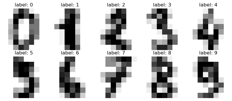
We construct a feedforward neural network using sklearn’s MLPClassifier. We will start with an architecture of two hidden layers. The default activation function is ReLU, and the output layer uses the softmax function.
The softmax function converts a vector of raw output scores (logits) \(\mathbf{z} = (z_1, \ldots, z_K)\), one per class, into a probability distribution over the \(K\) classes,
so that each \(p_k\) is nonnegative and the \(p_k\) sum to 1. In this setting, \(p_k\) is the network’s estimated probability that the input image belongs to digit class \(k\). We assign the predicted label by taking the class with the largest probability, \(\hat{y} = \arg\max_k p_k\). Below is the code.
from sklearn.datasets import load_digits
from sklearn.model_selection import train_test_split
from sklearn.preprocessing import StandardScaler
from sklearn.neural_network import MLPClassifier
from sklearn.metrics import accuracy_score

digits = load_digits()
X, y = digits.data, digits.target

X_train, X_test, y_train, y_test = train_test_split(
    X, y, test_size=0.2, random_state=42, stratify=y
)

# Scale features to zero mean / unit variance. MLPClassifier trains with
# gradient-based optimizers, which converge faster and more reliably
# when features are on a comparable scale -- here raw pixel values run
# 0-16, so this isn't as severe as for unscaled real-valued features,
# but it's cheap and still speeds up and stabilizes training.
scaler = StandardScaler()
X_train_scaled = scaler.fit_transform(X_train)
X_test_scaled = scaler.transform(X_test)

# hidden_layer_sizes=(100, 50) gives two hidden layers, since
# MLPClassifier's default of a single 100-unit layer doesn't match the
# two-hidden-layer architecture from the notes.
clf = MLPClassifier(
    hidden_layer_sizes=(100, 50),
    activation="relu",
    solver="adam",
    max_iter=200,
    random_state=42,
)
clf.fit(X_train_scaled, y_train)

y_pred = clf.predict(X_test_scaled)
acc = accuracy_score(y_test, y_pred)
print(f"Test accuracy: {acc:.4f}")
print(f"Number of epochs run: {clf.n_iter_} (max_iter={clf.max_iter})")
/opt/homebrew/Caskroom/miniforge/base/envs/sci_comp/lib/python3.13/site-packages/sklearn/utils/extmath.py:203: RuntimeWarning: divide by zero encountered in matmul
  ret = a @ b
/opt/homebrew/Caskroom/miniforge/base/envs/sci_comp/lib/python3.13/site-packages/sklearn/utils/extmath.py:203: RuntimeWarning: overflow encountered in matmul
  ret = a @ b
/opt/homebrew/Caskroom/miniforge/base/envs/sci_comp/lib/python3.13/site-packages/sklearn/utils/extmath.py:203: RuntimeWarning: invalid value encountered in matmul
  ret = a @ b
Test accuracy: 0.9778
Number of epochs run: 92 (max_iter=200)
/opt/homebrew/Caskroom/miniforge/base/envs/sci_comp/lib/python3.13/site-packages/sklearn/utils/extmath.py:203: RuntimeWarning: divide by zero encountered in matmul
  ret = a @ b
/opt/homebrew/Caskroom/miniforge/base/envs/sci_comp/lib/python3.13/site-packages/sklearn/utils/extmath.py:203: RuntimeWarning: overflow encountered in matmul
  ret = a @ b
/opt/homebrew/Caskroom/miniforge/base/envs/sci_comp/lib/python3.13/site-packages/sklearn/utils/extmath.py:203: RuntimeWarning: invalid value encountered in matmul
  ret = a @ b
We can now use sklearn’s cross-validation to experiment with different architectures.
from sklearn.model_selection import cross_val_score


# A few candidate architectures to compare, ranging from a single small
# hidden layer to deeper networks with more hidden layers. Note: this
# uses X_train, y_train from the earlier train/test split -- cross
# validation partitions the training set internally, so the held-out
# test set stays untouched until we pick a final architecture.
architectures = {
    "(50,)":        (50,),
    "(100,)":       (100,),
    "(100, 50)":    (100, 50),
    "(100, 100)":   (100, 100),
    "(50, 50, 50)": (50, 50, 50),
}

results = {}
for name, arch in architectures.items():
    clf = MLPClassifier(
        hidden_layer_sizes=arch,
        activation="relu",
        solver="adam",
        max_iter=200,
        random_state=42,
    )
    scores = cross_val_score(clf, X_train, y_train, cv=5)
    results[name] = scores
    print(f"{name:15s} mean accuracy = {scores.mean():.4f}  std = {scores.std():.4f}")

# Summary, sorted best to worst by mean CV accuracy
print("\nSummary of cross-validation results:")
print(f"{'Architecture':15s} {'Mean Accuracy':>15s} {'Std Dev':>10s}")
for name, scores in sorted(results.items(), key=lambda kv: kv[1].mean(), reverse=True):
    print(f"{name:15s} {scores.mean():15.4f} {scores.std():10.4f}")

best_arch = max(results, key=lambda k: results[k].mean())
print(f"\nBest architecture by mean CV accuracy: {best_arch} ({results[best_arch].mean():.4f})")
/opt/homebrew/Caskroom/miniforge/base/envs/sci_comp/lib/python3.13/site-packages/sklearn/utils/extmath.py:203: RuntimeWarning: divide by zero encountered in matmul
  ret = a @ b
/opt/homebrew/Caskroom/miniforge/base/envs/sci_comp/lib/python3.13/site-packages/sklearn/utils/extmath.py:203: RuntimeWarning: overflow encountered in matmul
  ret = a @ b
/opt/homebrew/Caskroom/miniforge/base/envs/sci_comp/lib/python3.13/site-packages/sklearn/utils/extmath.py:203: RuntimeWarning: invalid value encountered in matmul
  ret = a @ b
/opt/homebrew/Caskroom/miniforge/base/envs/sci_comp/lib/python3.13/site-packages/sklearn/utils/extmath.py:203: RuntimeWarning: divide by zero encountered in matmul
  ret = a @ b
/opt/homebrew/Caskroom/miniforge/base/envs/sci_comp/lib/python3.13/site-packages/sklearn/utils/extmath.py:203: RuntimeWarning: overflow encountered in matmul
  ret = a @ b
/opt/homebrew/Caskroom/miniforge/base/envs/sci_comp/lib/python3.13/site-packages/sklearn/utils/extmath.py:203: RuntimeWarning: invalid value encountered in matmul
  ret = a @ b
/opt/homebrew/Caskroom/miniforge/base/envs/sci_comp/lib/python3.13/site-packages/sklearn/utils/extmath.py:203: RuntimeWarning: divide by zero encountered in matmul
  ret = a @ b
/opt/homebrew/Caskroom/miniforge/base/envs/sci_comp/lib/python3.13/site-packages/sklearn/utils/extmath.py:203: RuntimeWarning: overflow encountered in matmul
  ret = a @ b
/opt/homebrew/Caskroom/miniforge/base/envs/sci_comp/lib/python3.13/site-packages/sklearn/utils/extmath.py:203: RuntimeWarning: invalid value encountered in matmul
  ret = a @ b
/opt/homebrew/Caskroom/miniforge/base/envs/sci_comp/lib/python3.13/site-packages/sklearn/utils/extmath.py:203: RuntimeWarning: divide by zero encountered in matmul
  ret = a @ b
/opt/homebrew/Caskroom/miniforge/base/envs/sci_comp/lib/python3.13/site-packages/sklearn/utils/extmath.py:203: RuntimeWarning: overflow encountered in matmul
  ret = a @ b
/opt/homebrew/Caskroom/miniforge/base/envs/sci_comp/lib/python3.13/site-packages/sklearn/utils/extmath.py:203: RuntimeWarning: invalid value encountered in matmul
  ret = a @ b
/opt/homebrew/Caskroom/miniforge/base/envs/sci_comp/lib/python3.13/site-packages/sklearn/utils/extmath.py:203: RuntimeWarning: divide by zero encountered in matmul
  ret = a @ b
/opt/homebrew/Caskroom/miniforge/base/envs/sci_comp/lib/python3.13/site-packages/sklearn/utils/extmath.py:203: RuntimeWarning: overflow encountered in matmul
  ret = a @ b
/opt/homebrew/Caskroom/miniforge/base/envs/sci_comp/lib/python3.13/site-packages/sklearn/utils/extmath.py:203: RuntimeWarning: invalid value encountered in matmul
  ret = a @ b
/opt/homebrew/Caskroom/miniforge/base/envs/sci_comp/lib/python3.13/site-packages/sklearn/utils/extmath.py:203: RuntimeWarning: divide by zero encountered in matmul
  ret = a @ b
/opt/homebrew/Caskroom/miniforge/base/envs/sci_comp/lib/python3.13/site-packages/sklearn/utils/extmath.py:203: RuntimeWarning: overflow encountered in matmul
  ret = a @ b
/opt/homebrew/Caskroom/miniforge/base/envs/sci_comp/lib/python3.13/site-packages/sklearn/utils/extmath.py:203: RuntimeWarning: invalid value encountered in matmul
  ret = a @ b
/opt/homebrew/Caskroom/miniforge/base/envs/sci_comp/lib/python3.13/site-packages/sklearn/utils/extmath.py:203: RuntimeWarning: divide by zero encountered in matmul
  ret = a @ b
/opt/homebrew/Caskroom/miniforge/base/envs/sci_comp/lib/python3.13/site-packages/sklearn/utils/extmath.py:203: RuntimeWarning: overflow encountered in matmul
  ret = a @ b
/opt/homebrew/Caskroom/miniforge/base/envs/sci_comp/lib/python3.13/site-packages/sklearn/utils/extmath.py:203: RuntimeWarning: invalid value encountered in matmul
  ret = a @ b
/opt/homebrew/Caskroom/miniforge/base/envs/sci_comp/lib/python3.13/site-packages/sklearn/utils/extmath.py:203: RuntimeWarning: divide by zero encountered in matmul
  ret = a @ b
/opt/homebrew/Caskroom/miniforge/base/envs/sci_comp/lib/python3.13/site-packages/sklearn/utils/extmath.py:203: RuntimeWarning: overflow encountered in matmul
  ret = a @ b
/opt/homebrew/Caskroom/miniforge/base/envs/sci_comp/lib/python3.13/site-packages/sklearn/utils/extmath.py:203: RuntimeWarning: invalid value encountered in matmul
  ret = a @ b
/opt/homebrew/Caskroom/miniforge/base/envs/sci_comp/lib/python3.13/site-packages/sklearn/utils/extmath.py:203: RuntimeWarning: divide by zero encountered in matmul
  ret = a @ b
/opt/homebrew/Caskroom/miniforge/base/envs/sci_comp/lib/python3.13/site-packages/sklearn/utils/extmath.py:203: RuntimeWarning: overflow encountered in matmul
  ret = a @ b
/opt/homebrew/Caskroom/miniforge/base/envs/sci_comp/lib/python3.13/site-packages/sklearn/utils/extmath.py:203: RuntimeWarning: invalid value encountered in matmul
  ret = a @ b
/opt/homebrew/Caskroom/miniforge/base/envs/sci_comp/lib/python3.13/site-packages/sklearn/utils/extmath.py:203: RuntimeWarning: divide by zero encountered in matmul
  ret = a @ b
/opt/homebrew/Caskroom/miniforge/base/envs/sci_comp/lib/python3.13/site-packages/sklearn/utils/extmath.py:203: RuntimeWarning: overflow encountered in matmul
  ret = a @ b
/opt/homebrew/Caskroom/miniforge/base/envs/sci_comp/lib/python3.13/site-packages/sklearn/utils/extmath.py:203: RuntimeWarning: invalid value encountered in matmul
  ret = a @ b
/opt/homebrew/Caskroom/miniforge/base/envs/sci_comp/lib/python3.13/site-packages/sklearn/utils/extmath.py:203: RuntimeWarning: divide by zero encountered in matmul
  ret = a @ b
/opt/homebrew/Caskroom/miniforge/base/envs/sci_comp/lib/python3.13/site-packages/sklearn/utils/extmath.py:203: RuntimeWarning: overflow encountered in matmul
  ret = a @ b
/opt/homebrew/Caskroom/miniforge/base/envs/sci_comp/lib/python3.13/site-packages/sklearn/utils/extmath.py:203: RuntimeWarning: invalid value encountered in matmul
  ret = a @ b
(50,) mean accuracy = 0.9610 std = 0.0111
/opt/homebrew/Caskroom/miniforge/base/envs/sci_comp/lib/python3.13/site-packages/sklearn/utils/extmath.py:203: RuntimeWarning: divide by zero encountered in matmul
  ret = a @ b
/opt/homebrew/Caskroom/miniforge/base/envs/sci_comp/lib/python3.13/site-packages/sklearn/utils/extmath.py:203: RuntimeWarning: overflow encountered in matmul
  ret = a @ b
/opt/homebrew/Caskroom/miniforge/base/envs/sci_comp/lib/python3.13/site-packages/sklearn/utils/extmath.py:203: RuntimeWarning: invalid value encountered in matmul
  ret = a @ b
/opt/homebrew/Caskroom/miniforge/base/envs/sci_comp/lib/python3.13/site-packages/sklearn/utils/extmath.py:203: RuntimeWarning: divide by zero encountered in matmul
  ret = a @ b
/opt/homebrew/Caskroom/miniforge/base/envs/sci_comp/lib/python3.13/site-packages/sklearn/utils/extmath.py:203: RuntimeWarning: overflow encountered in matmul
  ret = a @ b
/opt/homebrew/Caskroom/miniforge/base/envs/sci_comp/lib/python3.13/site-packages/sklearn/utils/extmath.py:203: RuntimeWarning: invalid value encountered in matmul
  ret = a @ b
/opt/homebrew/Caskroom/miniforge/base/envs/sci_comp/lib/python3.13/site-packages/sklearn/utils/extmath.py:203: RuntimeWarning: divide by zero encountered in matmul
  ret = a @ b
/opt/homebrew/Caskroom/miniforge/base/envs/sci_comp/lib/python3.13/site-packages/sklearn/utils/extmath.py:203: RuntimeWarning: overflow encountered in matmul
  ret = a @ b
/opt/homebrew/Caskroom/miniforge/base/envs/sci_comp/lib/python3.13/site-packages/sklearn/utils/extmath.py:203: RuntimeWarning: invalid value encountered in matmul
  ret = a @ b
/opt/homebrew/Caskroom/miniforge/base/envs/sci_comp/lib/python3.13/site-packages/sklearn/utils/extmath.py:203: RuntimeWarning: divide by zero encountered in matmul
  ret = a @ b
/opt/homebrew/Caskroom/miniforge/base/envs/sci_comp/lib/python3.13/site-packages/sklearn/utils/extmath.py:203: RuntimeWarning: overflow encountered in matmul
  ret = a @ b
/opt/homebrew/Caskroom/miniforge/base/envs/sci_comp/lib/python3.13/site-packages/sklearn/utils/extmath.py:203: RuntimeWarning: invalid value encountered in matmul
  ret = a @ b
/opt/homebrew/Caskroom/miniforge/base/envs/sci_comp/lib/python3.13/site-packages/sklearn/utils/extmath.py:203: RuntimeWarning: divide by zero encountered in matmul
  ret = a @ b
/opt/homebrew/Caskroom/miniforge/base/envs/sci_comp/lib/python3.13/site-packages/sklearn/utils/extmath.py:203: RuntimeWarning: overflow encountered in matmul
  ret = a @ b
/opt/homebrew/Caskroom/miniforge/base/envs/sci_comp/lib/python3.13/site-packages/sklearn/utils/extmath.py:203: RuntimeWarning: invalid value encountered in matmul
  ret = a @ b
/opt/homebrew/Caskroom/miniforge/base/envs/sci_comp/lib/python3.13/site-packages/sklearn/utils/extmath.py:203: RuntimeWarning: divide by zero encountered in matmul
  ret = a @ b
/opt/homebrew/Caskroom/miniforge/base/envs/sci_comp/lib/python3.13/site-packages/sklearn/utils/extmath.py:203: RuntimeWarning: overflow encountered in matmul
  ret = a @ b
/opt/homebrew/Caskroom/miniforge/base/envs/sci_comp/lib/python3.13/site-packages/sklearn/utils/extmath.py:203: RuntimeWarning: invalid value encountered in matmul
  ret = a @ b
/opt/homebrew/Caskroom/miniforge/base/envs/sci_comp/lib/python3.13/site-packages/sklearn/utils/extmath.py:203: RuntimeWarning: divide by zero encountered in matmul
  ret = a @ b
/opt/homebrew/Caskroom/miniforge/base/envs/sci_comp/lib/python3.13/site-packages/sklearn/utils/extmath.py:203: RuntimeWarning: overflow encountered in matmul
  ret = a @ b
/opt/homebrew/Caskroom/miniforge/base/envs/sci_comp/lib/python3.13/site-packages/sklearn/utils/extmath.py:203: RuntimeWarning: invalid value encountered in matmul
  ret = a @ b
/opt/homebrew/Caskroom/miniforge/base/envs/sci_comp/lib/python3.13/site-packages/sklearn/utils/extmath.py:203: RuntimeWarning: divide by zero encountered in matmul
  ret = a @ b
/opt/homebrew/Caskroom/miniforge/base/envs/sci_comp/lib/python3.13/site-packages/sklearn/utils/extmath.py:203: RuntimeWarning: overflow encountered in matmul
  ret = a @ b
/opt/homebrew/Caskroom/miniforge/base/envs/sci_comp/lib/python3.13/site-packages/sklearn/utils/extmath.py:203: RuntimeWarning: invalid value encountered in matmul
  ret = a @ b
/opt/homebrew/Caskroom/miniforge/base/envs/sci_comp/lib/python3.13/site-packages/sklearn/utils/extmath.py:203: RuntimeWarning: divide by zero encountered in matmul
  ret = a @ b
/opt/homebrew/Caskroom/miniforge/base/envs/sci_comp/lib/python3.13/site-packages/sklearn/utils/extmath.py:203: RuntimeWarning: overflow encountered in matmul
  ret = a @ b
/opt/homebrew/Caskroom/miniforge/base/envs/sci_comp/lib/python3.13/site-packages/sklearn/utils/extmath.py:203: RuntimeWarning: invalid value encountered in matmul
  ret = a @ b
/opt/homebrew/Caskroom/miniforge/base/envs/sci_comp/lib/python3.13/site-packages/sklearn/utils/extmath.py:203: RuntimeWarning: divide by zero encountered in matmul
  ret = a @ b
/opt/homebrew/Caskroom/miniforge/base/envs/sci_comp/lib/python3.13/site-packages/sklearn/utils/extmath.py:203: RuntimeWarning: overflow encountered in matmul
  ret = a @ b
/opt/homebrew/Caskroom/miniforge/base/envs/sci_comp/lib/python3.13/site-packages/sklearn/utils/extmath.py:203: RuntimeWarning: invalid value encountered in matmul
  ret = a @ b
(100,) mean accuracy = 0.9715 std = 0.0074
/opt/homebrew/Caskroom/miniforge/base/envs/sci_comp/lib/python3.13/site-packages/sklearn/utils/extmath.py:203: RuntimeWarning: divide by zero encountered in matmul
  ret = a @ b
/opt/homebrew/Caskroom/miniforge/base/envs/sci_comp/lib/python3.13/site-packages/sklearn/utils/extmath.py:203: RuntimeWarning: overflow encountered in matmul
  ret = a @ b
/opt/homebrew/Caskroom/miniforge/base/envs/sci_comp/lib/python3.13/site-packages/sklearn/utils/extmath.py:203: RuntimeWarning: invalid value encountered in matmul
  ret = a @ b
/opt/homebrew/Caskroom/miniforge/base/envs/sci_comp/lib/python3.13/site-packages/sklearn/utils/extmath.py:203: RuntimeWarning: divide by zero encountered in matmul
  ret = a @ b
/opt/homebrew/Caskroom/miniforge/base/envs/sci_comp/lib/python3.13/site-packages/sklearn/utils/extmath.py:203: RuntimeWarning: overflow encountered in matmul
  ret = a @ b
/opt/homebrew/Caskroom/miniforge/base/envs/sci_comp/lib/python3.13/site-packages/sklearn/utils/extmath.py:203: RuntimeWarning: invalid value encountered in matmul
  ret = a @ b
/opt/homebrew/Caskroom/miniforge/base/envs/sci_comp/lib/python3.13/site-packages/sklearn/utils/extmath.py:203: RuntimeWarning: divide by zero encountered in matmul
  ret = a @ b
/opt/homebrew/Caskroom/miniforge/base/envs/sci_comp/lib/python3.13/site-packages/sklearn/utils/extmath.py:203: RuntimeWarning: overflow encountered in matmul
  ret = a @ b
/opt/homebrew/Caskroom/miniforge/base/envs/sci_comp/lib/python3.13/site-packages/sklearn/utils/extmath.py:203: RuntimeWarning: invalid value encountered in matmul
  ret = a @ b
/opt/homebrew/Caskroom/miniforge/base/envs/sci_comp/lib/python3.13/site-packages/sklearn/utils/extmath.py:203: RuntimeWarning: divide by zero encountered in matmul
  ret = a @ b
/opt/homebrew/Caskroom/miniforge/base/envs/sci_comp/lib/python3.13/site-packages/sklearn/utils/extmath.py:203: RuntimeWarning: overflow encountered in matmul
  ret = a @ b
/opt/homebrew/Caskroom/miniforge/base/envs/sci_comp/lib/python3.13/site-packages/sklearn/utils/extmath.py:203: RuntimeWarning: invalid value encountered in matmul
  ret = a @ b
/opt/homebrew/Caskroom/miniforge/base/envs/sci_comp/lib/python3.13/site-packages/sklearn/utils/extmath.py:203: RuntimeWarning: divide by zero encountered in matmul
  ret = a @ b
/opt/homebrew/Caskroom/miniforge/base/envs/sci_comp/lib/python3.13/site-packages/sklearn/utils/extmath.py:203: RuntimeWarning: overflow encountered in matmul
  ret = a @ b
/opt/homebrew/Caskroom/miniforge/base/envs/sci_comp/lib/python3.13/site-packages/sklearn/utils/extmath.py:203: RuntimeWarning: invalid value encountered in matmul
  ret = a @ b
/opt/homebrew/Caskroom/miniforge/base/envs/sci_comp/lib/python3.13/site-packages/sklearn/utils/extmath.py:203: RuntimeWarning: divide by zero encountered in matmul
  ret = a @ b
/opt/homebrew/Caskroom/miniforge/base/envs/sci_comp/lib/python3.13/site-packages/sklearn/utils/extmath.py:203: RuntimeWarning: overflow encountered in matmul
  ret = a @ b
/opt/homebrew/Caskroom/miniforge/base/envs/sci_comp/lib/python3.13/site-packages/sklearn/utils/extmath.py:203: RuntimeWarning: invalid value encountered in matmul
  ret = a @ b
/opt/homebrew/Caskroom/miniforge/base/envs/sci_comp/lib/python3.13/site-packages/sklearn/utils/extmath.py:203: RuntimeWarning: divide by zero encountered in matmul
  ret = a @ b
/opt/homebrew/Caskroom/miniforge/base/envs/sci_comp/lib/python3.13/site-packages/sklearn/utils/extmath.py:203: RuntimeWarning: overflow encountered in matmul
  ret = a @ b
/opt/homebrew/Caskroom/miniforge/base/envs/sci_comp/lib/python3.13/site-packages/sklearn/utils/extmath.py:203: RuntimeWarning: invalid value encountered in matmul
  ret = a @ b
/opt/homebrew/Caskroom/miniforge/base/envs/sci_comp/lib/python3.13/site-packages/sklearn/utils/extmath.py:203: RuntimeWarning: divide by zero encountered in matmul
  ret = a @ b
/opt/homebrew/Caskroom/miniforge/base/envs/sci_comp/lib/python3.13/site-packages/sklearn/utils/extmath.py:203: RuntimeWarning: overflow encountered in matmul
  ret = a @ b
/opt/homebrew/Caskroom/miniforge/base/envs/sci_comp/lib/python3.13/site-packages/sklearn/utils/extmath.py:203: RuntimeWarning: invalid value encountered in matmul
  ret = a @ b
/opt/homebrew/Caskroom/miniforge/base/envs/sci_comp/lib/python3.13/site-packages/sklearn/utils/extmath.py:203: RuntimeWarning: divide by zero encountered in matmul
  ret = a @ b
/opt/homebrew/Caskroom/miniforge/base/envs/sci_comp/lib/python3.13/site-packages/sklearn/utils/extmath.py:203: RuntimeWarning: overflow encountered in matmul
  ret = a @ b
/opt/homebrew/Caskroom/miniforge/base/envs/sci_comp/lib/python3.13/site-packages/sklearn/utils/extmath.py:203: RuntimeWarning: invalid value encountered in matmul
  ret = a @ b
/opt/homebrew/Caskroom/miniforge/base/envs/sci_comp/lib/python3.13/site-packages/sklearn/utils/extmath.py:203: RuntimeWarning: divide by zero encountered in matmul
  ret = a @ b
/opt/homebrew/Caskroom/miniforge/base/envs/sci_comp/lib/python3.13/site-packages/sklearn/utils/extmath.py:203: RuntimeWarning: overflow encountered in matmul
  ret = a @ b
/opt/homebrew/Caskroom/miniforge/base/envs/sci_comp/lib/python3.13/site-packages/sklearn/utils/extmath.py:203: RuntimeWarning: invalid value encountered in matmul
  ret = a @ b
/opt/homebrew/Caskroom/miniforge/base/envs/sci_comp/lib/python3.13/site-packages/sklearn/utils/extmath.py:203: RuntimeWarning: divide by zero encountered in matmul
  ret = a @ b
/opt/homebrew/Caskroom/miniforge/base/envs/sci_comp/lib/python3.13/site-packages/sklearn/utils/extmath.py:203: RuntimeWarning: overflow encountered in matmul
  ret = a @ b
/opt/homebrew/Caskroom/miniforge/base/envs/sci_comp/lib/python3.13/site-packages/sklearn/utils/extmath.py:203: RuntimeWarning: invalid value encountered in matmul
  ret = a @ b
/opt/homebrew/Caskroom/miniforge/base/envs/sci_comp/lib/python3.13/site-packages/sklearn/utils/extmath.py:203: RuntimeWarning: divide by zero encountered in matmul
  ret = a @ b
/opt/homebrew/Caskroom/miniforge/base/envs/sci_comp/lib/python3.13/site-packages/sklearn/utils/extmath.py:203: RuntimeWarning: overflow encountered in matmul
  ret = a @ b
/opt/homebrew/Caskroom/miniforge/base/envs/sci_comp/lib/python3.13/site-packages/sklearn/utils/extmath.py:203: RuntimeWarning: invalid value encountered in matmul
  ret = a @ b
(100, 50) mean accuracy = 0.9659 std = 0.0081
/opt/homebrew/Caskroom/miniforge/base/envs/sci_comp/lib/python3.13/site-packages/sklearn/utils/extmath.py:203: RuntimeWarning: divide by zero encountered in matmul
  ret = a @ b
/opt/homebrew/Caskroom/miniforge/base/envs/sci_comp/lib/python3.13/site-packages/sklearn/utils/extmath.py:203: RuntimeWarning: overflow encountered in matmul
  ret = a @ b
/opt/homebrew/Caskroom/miniforge/base/envs/sci_comp/lib/python3.13/site-packages/sklearn/utils/extmath.py:203: RuntimeWarning: invalid value encountered in matmul
  ret = a @ b
/opt/homebrew/Caskroom/miniforge/base/envs/sci_comp/lib/python3.13/site-packages/sklearn/utils/extmath.py:203: RuntimeWarning: divide by zero encountered in matmul
  ret = a @ b
/opt/homebrew/Caskroom/miniforge/base/envs/sci_comp/lib/python3.13/site-packages/sklearn/utils/extmath.py:203: RuntimeWarning: overflow encountered in matmul
  ret = a @ b
/opt/homebrew/Caskroom/miniforge/base/envs/sci_comp/lib/python3.13/site-packages/sklearn/utils/extmath.py:203: RuntimeWarning: invalid value encountered in matmul
  ret = a @ b
/opt/homebrew/Caskroom/miniforge/base/envs/sci_comp/lib/python3.13/site-packages/sklearn/utils/extmath.py:203: RuntimeWarning: divide by zero encountered in matmul
  ret = a @ b
/opt/homebrew/Caskroom/miniforge/base/envs/sci_comp/lib/python3.13/site-packages/sklearn/utils/extmath.py:203: RuntimeWarning: overflow encountered in matmul
  ret = a @ b
/opt/homebrew/Caskroom/miniforge/base/envs/sci_comp/lib/python3.13/site-packages/sklearn/utils/extmath.py:203: RuntimeWarning: invalid value encountered in matmul
  ret = a @ b
/opt/homebrew/Caskroom/miniforge/base/envs/sci_comp/lib/python3.13/site-packages/sklearn/utils/extmath.py:203: RuntimeWarning: divide by zero encountered in matmul
  ret = a @ b
/opt/homebrew/Caskroom/miniforge/base/envs/sci_comp/lib/python3.13/site-packages/sklearn/utils/extmath.py:203: RuntimeWarning: overflow encountered in matmul
  ret = a @ b
/opt/homebrew/Caskroom/miniforge/base/envs/sci_comp/lib/python3.13/site-packages/sklearn/utils/extmath.py:203: RuntimeWarning: invalid value encountered in matmul
  ret = a @ b
/opt/homebrew/Caskroom/miniforge/base/envs/sci_comp/lib/python3.13/site-packages/sklearn/utils/extmath.py:203: RuntimeWarning: divide by zero encountered in matmul
  ret = a @ b
/opt/homebrew/Caskroom/miniforge/base/envs/sci_comp/lib/python3.13/site-packages/sklearn/utils/extmath.py:203: RuntimeWarning: overflow encountered in matmul
  ret = a @ b
/opt/homebrew/Caskroom/miniforge/base/envs/sci_comp/lib/python3.13/site-packages/sklearn/utils/extmath.py:203: RuntimeWarning: invalid value encountered in matmul
  ret = a @ b
/opt/homebrew/Caskroom/miniforge/base/envs/sci_comp/lib/python3.13/site-packages/sklearn/utils/extmath.py:203: RuntimeWarning: divide by zero encountered in matmul
  ret = a @ b
/opt/homebrew/Caskroom/miniforge/base/envs/sci_comp/lib/python3.13/site-packages/sklearn/utils/extmath.py:203: RuntimeWarning: overflow encountered in matmul
  ret = a @ b
/opt/homebrew/Caskroom/miniforge/base/envs/sci_comp/lib/python3.13/site-packages/sklearn/utils/extmath.py:203: RuntimeWarning: invalid value encountered in matmul
  ret = a @ b
/opt/homebrew/Caskroom/miniforge/base/envs/sci_comp/lib/python3.13/site-packages/sklearn/utils/extmath.py:203: RuntimeWarning: divide by zero encountered in matmul
  ret = a @ b
/opt/homebrew/Caskroom/miniforge/base/envs/sci_comp/lib/python3.13/site-packages/sklearn/utils/extmath.py:203: RuntimeWarning: overflow encountered in matmul
  ret = a @ b
/opt/homebrew/Caskroom/miniforge/base/envs/sci_comp/lib/python3.13/site-packages/sklearn/utils/extmath.py:203: RuntimeWarning: invalid value encountered in matmul
  ret = a @ b
/opt/homebrew/Caskroom/miniforge/base/envs/sci_comp/lib/python3.13/site-packages/sklearn/utils/extmath.py:203: RuntimeWarning: divide by zero encountered in matmul
  ret = a @ b
/opt/homebrew/Caskroom/miniforge/base/envs/sci_comp/lib/python3.13/site-packages/sklearn/utils/extmath.py:203: RuntimeWarning: overflow encountered in matmul
  ret = a @ b
/opt/homebrew/Caskroom/miniforge/base/envs/sci_comp/lib/python3.13/site-packages/sklearn/utils/extmath.py:203: RuntimeWarning: invalid value encountered in matmul
  ret = a @ b
(100, 100) mean accuracy = 0.9694 std = 0.0135
/opt/homebrew/Caskroom/miniforge/base/envs/sci_comp/lib/python3.13/site-packages/sklearn/utils/extmath.py:203: RuntimeWarning: divide by zero encountered in matmul
  ret = a @ b
/opt/homebrew/Caskroom/miniforge/base/envs/sci_comp/lib/python3.13/site-packages/sklearn/utils/extmath.py:203: RuntimeWarning: overflow encountered in matmul
  ret = a @ b
/opt/homebrew/Caskroom/miniforge/base/envs/sci_comp/lib/python3.13/site-packages/sklearn/utils/extmath.py:203: RuntimeWarning: invalid value encountered in matmul
  ret = a @ b
/opt/homebrew/Caskroom/miniforge/base/envs/sci_comp/lib/python3.13/site-packages/sklearn/utils/extmath.py:203: RuntimeWarning: divide by zero encountered in matmul
  ret = a @ b
/opt/homebrew/Caskroom/miniforge/base/envs/sci_comp/lib/python3.13/site-packages/sklearn/utils/extmath.py:203: RuntimeWarning: overflow encountered in matmul
  ret = a @ b
/opt/homebrew/Caskroom/miniforge/base/envs/sci_comp/lib/python3.13/site-packages/sklearn/utils/extmath.py:203: RuntimeWarning: invalid value encountered in matmul
  ret = a @ b
/opt/homebrew/Caskroom/miniforge/base/envs/sci_comp/lib/python3.13/site-packages/sklearn/utils/extmath.py:203: RuntimeWarning: divide by zero encountered in matmul
  ret = a @ b
/opt/homebrew/Caskroom/miniforge/base/envs/sci_comp/lib/python3.13/site-packages/sklearn/utils/extmath.py:203: RuntimeWarning: overflow encountered in matmul
  ret = a @ b
/opt/homebrew/Caskroom/miniforge/base/envs/sci_comp/lib/python3.13/site-packages/sklearn/utils/extmath.py:203: RuntimeWarning: invalid value encountered in matmul
  ret = a @ b
/opt/homebrew/Caskroom/miniforge/base/envs/sci_comp/lib/python3.13/site-packages/sklearn/utils/extmath.py:203: RuntimeWarning: divide by zero encountered in matmul
  ret = a @ b
/opt/homebrew/Caskroom/miniforge/base/envs/sci_comp/lib/python3.13/site-packages/sklearn/utils/extmath.py:203: RuntimeWarning: overflow encountered in matmul
  ret = a @ b
/opt/homebrew/Caskroom/miniforge/base/envs/sci_comp/lib/python3.13/site-packages/sklearn/utils/extmath.py:203: RuntimeWarning: invalid value encountered in matmul
  ret = a @ b
/opt/homebrew/Caskroom/miniforge/base/envs/sci_comp/lib/python3.13/site-packages/sklearn/utils/extmath.py:203: RuntimeWarning: divide by zero encountered in matmul
  ret = a @ b
/opt/homebrew/Caskroom/miniforge/base/envs/sci_comp/lib/python3.13/site-packages/sklearn/utils/extmath.py:203: RuntimeWarning: overflow encountered in matmul
  ret = a @ b
/opt/homebrew/Caskroom/miniforge/base/envs/sci_comp/lib/python3.13/site-packages/sklearn/utils/extmath.py:203: RuntimeWarning: invalid value encountered in matmul
  ret = a @ b
/opt/homebrew/Caskroom/miniforge/base/envs/sci_comp/lib/python3.13/site-packages/sklearn/utils/extmath.py:203: RuntimeWarning: divide by zero encountered in matmul
  ret = a @ b
/opt/homebrew/Caskroom/miniforge/base/envs/sci_comp/lib/python3.13/site-packages/sklearn/utils/extmath.py:203: RuntimeWarning: overflow encountered in matmul
  ret = a @ b
/opt/homebrew/Caskroom/miniforge/base/envs/sci_comp/lib/python3.13/site-packages/sklearn/utils/extmath.py:203: RuntimeWarning: invalid value encountered in matmul
  ret = a @ b
/opt/homebrew/Caskroom/miniforge/base/envs/sci_comp/lib/python3.13/site-packages/sklearn/utils/extmath.py:203: RuntimeWarning: divide by zero encountered in matmul
  ret = a @ b
/opt/homebrew/Caskroom/miniforge/base/envs/sci_comp/lib/python3.13/site-packages/sklearn/utils/extmath.py:203: RuntimeWarning: overflow encountered in matmul
  ret = a @ b
/opt/homebrew/Caskroom/miniforge/base/envs/sci_comp/lib/python3.13/site-packages/sklearn/utils/extmath.py:203: RuntimeWarning: invalid value encountered in matmul
  ret = a @ b
/opt/homebrew/Caskroom/miniforge/base/envs/sci_comp/lib/python3.13/site-packages/sklearn/utils/extmath.py:203: RuntimeWarning: divide by zero encountered in matmul
  ret = a @ b
/opt/homebrew/Caskroom/miniforge/base/envs/sci_comp/lib/python3.13/site-packages/sklearn/utils/extmath.py:203: RuntimeWarning: overflow encountered in matmul
  ret = a @ b
/opt/homebrew/Caskroom/miniforge/base/envs/sci_comp/lib/python3.13/site-packages/sklearn/utils/extmath.py:203: RuntimeWarning: invalid value encountered in matmul
  ret = a @ b
(50, 50, 50)    mean accuracy = 0.9617  std = 0.0119

Summary of cross-validation results:
Architecture      Mean Accuracy    Std Dev
(100,)                   0.9715     0.0074
(100, 100)               0.9694     0.0135
(100, 50)                0.9659     0.0081
(50, 50, 50)             0.9617     0.0119
(50,)                    0.9610     0.0111

Best architecture by mean CV accuracy: (100,) (0.9715)
/opt/homebrew/Caskroom/miniforge/base/envs/sci_comp/lib/python3.13/site-packages/sklearn/utils/extmath.py:203: RuntimeWarning: divide by zero encountered in matmul
  ret = a @ b
/opt/homebrew/Caskroom/miniforge/base/envs/sci_comp/lib/python3.13/site-packages/sklearn/utils/extmath.py:203: RuntimeWarning: overflow encountered in matmul
  ret = a @ b
/opt/homebrew/Caskroom/miniforge/base/envs/sci_comp/lib/python3.13/site-packages/sklearn/utils/extmath.py:203: RuntimeWarning: invalid value encountered in matmul
  ret = a @ b