6.2. Convolution and Correlation#
The discrete convolution operation, denoted by \(*\), takes two digital signals, \(f\) and \(g\), to create a third signal given by
where \(n\) indexes the discrete domain. For finite sequences of length \(N\), the indices are typically evaluated modulo \(N\), yielding circular convolution.
The Convolution Theorem (see below) establishes that convolution in the time domain is equivalent to point-wise multiplication in the frequency domain, \(\mathcal{F}\{f * g\} = \mathcal{F}\{f\} \cdot \mathcal{F}\{g\}\), allowing large discrete convolutions to be computed efficiently in \(\mathcal{O}(N \log N)\) operations using the Fast Fourier Transform.
To understand the mechanics of discrete linear convolution, we construct the algorithm explicitly. Given two finite discrete signals \(f\) of length \(N_1\) and \(g\) of length \(N_2\), their linear convolution \(s = f * g\) produces a new signal \(s\) of total length \(M = N_1 + N_2 - 1\). The \(n\)-th element of the output sequence is given by the discrete sum
where \(n \in \{0, 1, \dots, M - 1\}\). The summation index \(k\) ranges over valid overlap indices bounded by \(k_{\text{min}} = \max(0, n - N_2 + 1)\) and \(k_{\text{max}} = \min(n, N_1 - 1)\).
To visualize how the terms slide past one another, consider two sequences of length \(N_1 = 4\) and \(N_2 = 4\), with indices \(k \in \{0, 1, 2, 3\}\). The full convolution sequence consists of \(M = 4 + 4 - 1 = 7\) terms, evaluated symbolically index-by-index:
Notice how \(g\) is reversed with respect to its indexing and shifts across \(f\) as \(n\) increases from \(0\) to \(6\).
import numpy as np
from numpy.fft import fft, ifft, fftfreq, fftshift
from numpy import pi, cos, sin, exp
from numpy import convolve

%matplotlib inline
import matplotlib.pyplot as plt
def brute_force_convolve(f, g):
    """Compute 1D discrete linear convolution via explicit summation bounds."""
    n1 = f.size
    n2 = g.size
    m = n1 + n2 - 1

    s = np.zeros(m)

    for n in range(m):
        # Determine valid summation bounds for non-zero overlap
        kmin = max(0, n - n2 + 1)
        kmax = min(n, n1 - 1)

        for k in range(kmin, kmax + 1):
            s[n] += f[k] * g[n - k]

    return s


# Define test input sequences
f = np.arange(1, 5)  # [1, 2, 3, 4]
g = np.arange(5, 9)  # [5, 6, 7, 8]

# 1. Compute via custom explicit loop function
s_loop = brute_force_convolve(f, g)

# 2. Compute via explicit element-by-element expansion
s_explicit = np.zeros(7)
s_explicit[0] = f[0] * g[0]
s_explicit[1] = f[0] * g[1] + f[1] * g[0]
s_explicit[2] = f[0] * g[2] + f[1] * g[1] + f[2] * g[0]
s_explicit[3] = f[0] * g[3] + f[1] * g[2] + f[2] * g[1] + f[3] * g[0]
s_explicit[4] = f[1] * g[3] + f[2] * g[2] + f[3] * g[1]
s_explicit[5] = f[2] * g[3] + f[3] * g[2]
s_explicit[6] = f[3] * g[3]

# 3. Compute via NumPy built-in function
s_numpy = np.convolve(f, g)

# Display results
print("Brute-Force Loop:      ", s_loop)
print("Explicit Term-by-Term: ", s_explicit)
print("NumPy np.convolve:     ", s_numpy)
print("Matches NumPy?:        ", np.allclose(s_loop, s_numpy))
Brute-Force Loop:       [ 5. 16. 34. 60. 61. 52. 32.]
Explicit Term-by-Term:  [ 5. 16. 34. 60. 61. 52. 32.]
NumPy np.convolve:      [ 5 16 34 60 61 52 32]
Matches NumPy?:         True
6.2.1. Edge Handling and Boundary Modes in np.convolve#
When computing the linear convolution of two discrete sequences \(f\) of length \(N_1\) and \(g\) of length \(N_2\), the full output sequence has length \(M = N_1 + N_2 - 1\). In practical applications, however, it is often desirable to restrict the output domain based on boundary conditions and overlap. NumPy’s np.convolve(f, g, mode=...) function provides three options to control the boundary evaluation: 'full', 'same', and 'valid'.
6.2.1.1. 1. Full Mode (mode='full')#
The default setting is mode='full', which returns the complete linear convolution of length \(M = N_1 + N_2 - 1\). This mode evaluates the summation at every index \(n\) where the two sequences have non-zero overlap, including partial overlap at the boundary edges. The output elements are given by
This mode is necessary when preserving all boundary effects and total signal energy is required.
6.2.1.2. 2. Same Mode (mode='same')#
The mode='same' setting returns a centered slice of the full convolution that matches the length of the first input sequence, \(N_{\text{out}} = \max(N_1, N_2) = N_1\) (assuming \(N_1 \ge N_2\)). The output values correspond to
This mode is widely used in filtering and smoothing time series because it preserves the original array dimension and keeps the filtered signal temporally aligned with the input data.
6.2.1.3. 3. Valid Mode (mode='valid')#
The mode='valid' setting restricts evaluation strictly to indices where the two sequences overlap completely without zero-padding or boundary extension. For sequences of lengths \(N_1\) and \(N_2\) (with \(N_1 \ge N_2\)), the resulting output has length \(N_{\text{out}} = N_1 - N_2 + 1\), defined by
Because edge regions with incomplete kernel overlap are excluded entirely, mode='valid' guarantees that every computed output point is free from boundary artifact distortion.
6.2.2. The Discrete Convolution Theorem#
The Discrete Convolution Theorem states that the discrete Fourier transform of the circular convolution of two sequences equals the point-wise product of their individual discrete Fourier transforms. Expressed mathematically, if \(h[n] = (f * g)[n]\) for finite sequences of length \(N\), then
where \(\mathcal{F}\) denotes the discrete Fourier transform operator.
Let \(f[n]\) and \(g[n]\) be periodic sequences of length \(N\). The discrete Fourier transform of their circular convolution is defined as
Interchanging the order of summation yields
Applying the index substitution \(r = (n - k) \pmod N\), where \(n = r + k\), the inner summation transforms over one full period \(r \in \{0, 1, \dots, N-1\}\) to
Substituting this back into the outer summation gives
Factoring out the inner sum, which is independent of \(k\), separates the expression into two independent discrete Fourier transforms,
Recognizing each summation as the definition of the individual DFTs completes the proof,
6.2.2.1. Convolution via the Fast Fourier Transform#
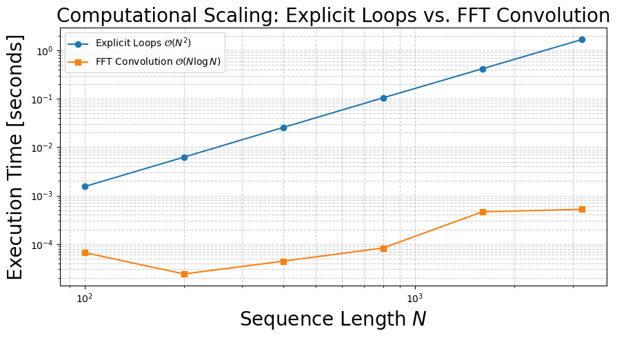
The Convolution Theorem provides an efficient computational “shortcut” for evaluating discrete convolutions. By transforming time-domain or spatial-domain signals into the frequency domain, the computationally intensive \(\mathcal{O}(N^2)\) summation reduces to a simple point-wise multiplication requiring only \(\mathcal{O}(N)\) operations. To convolve two finite sequences \(f\) and \(g\) using this theorem, one pads both signals to length \(N_{\text{out}} = N_1 + N_2 - 1\) with zeros to prevent circular aliasing, evaluates their individual discrete Fourier transforms via the Fast Fourier Transform (FFT), multiplies the resulting spectra point-by-point, and applies the inverse FFT (IFFT) to return to the physical domain. Because the FFT algorithm runs in \(\mathcal{O}(N \log N)\) time, this approach offers dramatic performance gains for large sequences.
Below, we implement this FFT-based convolution in Python and verify that its output matches NumPy’s built-in np.convolve.
def fft_convolve(f, g):
    """Compute 1D linear convolution via FFT in O(N log N) time."""
    n_out = f.size + g.size - 1

    # Zero-pad to avoid circular overlap and compute FFTs
    F = np.fft.fft(f, n=n_out)
    G = np.fft.fft(g, n=n_out)

    # Point-wise multiplication in frequency domain and inverse transform
    return np.real(np.fft.ifft(F * G))


# Generate sample sequences
f = np.arange(1, 5)
g = np.arange(5, 9)

# Compare results
s_fft = fft_convolve(f, g)
s_numpy = np.convolve(f, g)

print("FFT Convolution: ", s_fft)
print("np.convolve:     ", s_numpy)
print("Matches NumPy?:  ", np.allclose(s_fft, s_numpy))
FFT Convolution:  [ 5. 16. 34. 60. 61. 52. 32.]
np.convolve:      [ 5 16 34 60 61 52 32]
Matches NumPy?:   True
Below the computational effort of brute force convolution is compared to convolution by FFT.
import time

def brute_force_convolve(f, g):
    """Explicit O(N^2) linear convolution using loops."""
    n1 = f.size
    n2 = g.size
    m = n1 + n2 - 1
    s = np.zeros(m)

    for n in range(m):
        kmin = max(0, n - n2 + 1)
        kmax = min(n, n1 - 1)
        for k in range(kmin, kmax + 1):
            s[n] += f[k] * g[n - k]

    return s


# Array sizes to test
sizes = [100, 200, 400, 800, 1600, 3200]

times_brute = []
times_fft = []

for N in sizes:
    f = np.random.randn(N)
    g = np.random.randn(N)

    # Benchmark Brute-Force O(N^2)
    start = time.perf_counter()
    _ = brute_force_convolve(f, g)
    times_brute.append(time.perf_counter() - start)

    # Benchmark Fast Convolution O(N log N)
    start = time.perf_counter()
    _ = fft_convolve(f, g)
    times_fft.append(time.perf_counter() - start)

# Plotting performance scaling
plt.figure(figsize=(9, 5))
plt.plot(sizes, times_brute, "o-", label=r"Explicit Loops $\mathcal{O}(N^2)$")
plt.plot(sizes, times_fft, "s-", label=r"FFT Convolution $\mathcal{O}(N \log N)$")

plt.xlabel("Sequence Length $N$", size=20)
plt.ylabel("Execution Time [seconds]",size=20)
plt.title("Computational Scaling: Explicit Loops vs. FFT Convolution",size=20)
plt.yscale("log")
plt.xscale("log")
plt.grid(True, which="both", linestyle="--", alpha=0.6)
plt.legend()
plt.tight_layout()
plt.show()
6.2.2.2. Moving Average via Convolution#
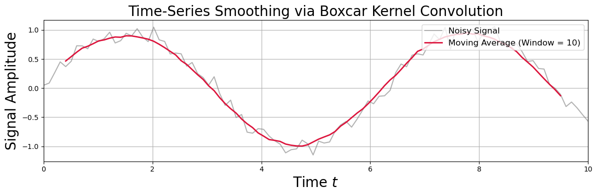
In, yet, another application, discrete convolution can be used to construct a moving average filter to smooth noisy time-series data. A moving average is implemented by convolving a discrete signal \(f[n]\) with a boxcar kernel (a normalized unit window function) of length \(W\), defined as
Convolving a signal with this kernel computes an unweighted local arithmetic mean at each sliding window position. The parameter \(W\) controls the degree of smoothing: a larger window size suppresses high-frequency noise more aggressively at the expense of blurring rapid signal transitions and truncating edge values.
Below, we demonstrate a moving average filter applied to a noisy sinusoidal signal using NumPy’s np.convolve.
# Set random seed for reproducibility
np.random.seed(42)


def moving_average(signal, window_size):
    """Compute moving average filter using 1D discrete convolution."""
    kernel = np.ones(window_size) / window_size
    return np.convolve(signal, kernel, mode="valid")


# Generate synthetic noisy signal
t = np.linspace(0, 10, 100)
signal = np.sin(t) + np.random.normal(0, 0.1, size=t.shape)

# Set window size for moving average
w_size = 10

# Perform moving average
smoothed = moving_average(signal, w_size)

# Align time array for 'valid' convolution mode (centers the window)
i_start = (w_size - 1) // 2
i_end = i_start + smoothed.size
t_smoothed = t[i_start:i_end]

# Plot original and smoothed signals
fig = plt.figure(figsize=(12, 4))
ax = fig.add_subplot()

ax.plot(t, signal, color="gray", alpha=0.6, label="Noisy Signal")
ax.plot(
    t_smoothed,
    smoothed,
    color="crimson",
    linewidth=2.0,
    label=f"Moving Average (Window = {w_size})",
)

ax.set_xlim(0, 10)
ax.set_xlabel("Time $t$", size=20)
ax.set_ylabel("Signal Amplitude", size=20)
ax.set_title("Time-Series Smoothing via Boxcar Kernel Convolution", size=20)
ax.grid(True)
ax.legend(loc="upper right", fontsize="large")

plt.tight_layout()
plt.show()
6.2.3. Correlation#
An operation similar in mathematical structure to convolution is correlation. The discrete cross-correlation between two signals \(f\) and \(g\) is defined as
where \(f^*\) denotes the complex conjugate of \(f\), and \(n\) represents the relative shift or lag between the two signals. Unlike convolution, where one signal is time-reversed before shifting, correlation preserves the time orientation of both signals.
When a signal is correlated with itself, the operation is called autocorrelation, given by
which quantifies the degree of self-similarity in a signal across various time delays \(n\).
Cross-correlation provides a quantitative measure of how similar two signals are as a function of the relative displacement of one relative to the other.
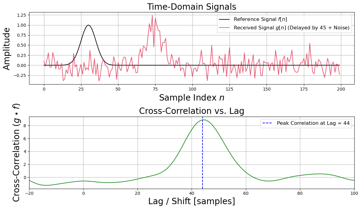
An application of cross-correlation is finding the unknown relative time delay between two signals. Suppose a known reference signal \(f[n]\) is transmitted, and a receiver records a delayed, noisy version \(g[n] = f[n - n_0] + \text{noise}\). The cross-correlation \((g \star f)[n]\) reaches its maximum peak precisely at lag \(n = n_0\), revealing the precise time of arrival.
Below, we construct a localized pulse signal, apply a time lag with additive Gaussian noise, and use np.correlate to recover the true delay.
# Set random seed for reproducibility
np.random.seed(42)

# --- 1. Generate Signal and Delayed Echo ---
N = 200
t = np.arange(N)

# Reference signal: a Gaussian-windowed pulse
f = np.exp(-0.5 * ((t - 30) / 5) ** 2)

# True time delay (shift)
true_delay = 45
print("The constructed delay is, ", true_delay)

# Received signal: delayed version of f + zero-mean Gaussian noise
g = np.roll(f, true_delay) + np.random.normal(0, 0.2, size=N)

# --- 2. Compute Cross-Correlation ---
# mode='full' computes cross-correlation at all possible relative lags
corr = np.correlate(g, f, mode="full")

# Generate lag indices corresponding to mode='full' output
lags = np.arange(-N + 1, N)

# Estimated delay corresponds to the lag value where correlation is maximized
estimated_delay = lags[np.argmax(corr)]

print(f"True Time Delay:      {true_delay} samples")
print(f"Estimated Time Delay: {estimated_delay} samples")

# --- 3. Visualization ---
fig, axes = plt.subplots(2, 1, figsize=(12, 7), sharex=False)

# Time Domain Signals
axes[0].plot(t, f, color="black", label="Reference Signal $f[n]$")
axes[0].plot(
    t,
    g,
    color="crimson",
    alpha=0.7,
    label=f"Received Signal $g[n]$ (Delayed by {true_delay} + Noise)",
)
axes[0].set_xlabel(r"Sample Index $n$", size=20)
axes[0].set_ylabel("Amplitude",size=20)
axes[0].set_title("Time-Domain Signals", size=20)
axes[0].legend(loc="upper right", fontsize="large")
axes[0].grid(True)

# Cross-Correlation Sequence
axes[1].plot(lags, corr, color="forestgreen", linewidth=1.5)
axes[1].axvline(
    estimated_delay,
    color="blue",
    linestyle="--",
    label=f"Peak Correlation at Lag = {estimated_delay}",
)
axes[1].set_xlim(-20, 100)  # Focus on reasonable positive lags
axes[1].set_xlabel("Lag / Shift [samples]", size=20)
axes[1].set_ylabel(r"Cross-Correlation $(g \star f)$", size=20)
axes[1].set_title("Cross-Correlation vs. Lag", size=20)
axes[1].legend(loc="upper right", fontsize="large")
axes[1].grid(True)

plt.tight_layout()
The constructed delay is,  45
True Time Delay:      45 samples
Estimated Time Delay: 44 samples