2.3. Psuedo Code Exercise#
Writing code from psuedo code is very important, it will be one of the major themes of this course. In your career you might read a research paper with an algorithm in psuedo code, you need to have the ability to write that algoritm into code. Or, perhaps, you need to explain an algorithm to a group of people who do not all code in the same programing language. You will need your explanation in psuedo code. More than any other reason, writing code from psuedo code forces you to think about how the algorithm works, hence it will boost your intution for the method.
In this note, instead of focusing on a traditional machine learning algorithm, we will look at what is called a random walk. The benefit to studying the the random walk is vast, a few reasons are: 1) it is simple and does not need much math, and it has much applicaiton to real world phenomena.
2.3.1. Random Walk#
If you are unfamiliar with some of the Python functionality needed, for example random numbers and arrays, then jump ahead to those relevant chapters.
In this exercise we will look at a two-dimensional random walk. A random walk is a mathematical model that describes a path consisting of a succession of random steps. In a 2D random walk, a particle starts at the origin and at each time step moves one unit in a randomly chosen direction (up, down, left, or right).
Random walks have applications in diffusion modeling, for example in physics (Brownian motion), biology (animal foraging patterns), and financial modeling (stock price movements). They help us understand how particles spread out over time and model various stochastic processes in nature.
2.3.1.1. NumPy’s Random Choice#
We will need to generate steps of unit length. To do so, we can use the random choice function in NumPy. The random choice function chooses a random element from a multi-element data structure, for example, a list or an array. Here is an example of randomly choosing between -1 and 1 (representing steps of unit length in either direction):
steps = [-1, 1]
result = np.random.choice(steps)
print(result)
Each time you call random choice, you will get a different result, unless you have fixed the random seed. You could observe this by using a loop:
for i in range(10):
result = np.random.choice(steps)
print(result)
By default, the random choice function assigns equal probability to each outcome. You can weight each element by a probability. For example, let us say that we want 65% of the outcomes to be 1 and 35% to be -1. Here is code to do that:
steps = [-1, 1]
probability = [0.35, 0.65]
result = np.random.choice(steps, p=probability)
print(result)
Question
When declaring probabilities for each element, what should those probabilities add up to?
Answer: The probabilities should add up to 1.0 (or 100%). This is a fundamental requirement in probability theory - all possible outcomes must sum to 1. In our example above, 0.35 + 0.65 = 1.0, which is correct. If the probabilities don’t sum to 1, NumPy will raise an error.
Exercise
Write code to compute 10,000 outcomes of random choices between -1 and 1, weighted with respective probabilities of 30% and 70%. Collect the results into an array of size 10,000. Count the number of occurrences of -1 and 1 and find the experimental fractions for each occurrence, i.e., the number of occurrences divided by the total number of samples. Your results should be close to 0.3 and 0.7.
Answer
import numpy as np
# Define the problem parameters
n = 10000 # Number of random samples to generate
steps = [-1, 1] # Possible outcomes
probability = [0.3, 0.7] # Probabilities for -1 and 1 respectively
# Create array to store results
results = np.zeros(n, dtype=int)
# Generate random choices with specified probabilities
for i in range(n):
results[i] = np.random.choice(steps, p=probability)
# Count occurrences of each outcome
n1 = np.sum(results == -1) # Count of -1 outcomes
n2 = np.sum(results == 1) # Count of 1 outcomes
# Calculate experimental fractions
f1 = n1 / n # Fraction of -1 outcomes
f2 = n2 / n # Fraction of 1 outcomes
# Display results
print(f"Fraction of -1 outcomes: {f1:.3f} (expected: 0.3)")
print(f"Fraction of 1 outcomes: {f2:.3f} (expected: 0.7)")
print(f"Total samples: {n1 + n2}")
Below is pseudocode for a two-dimensional random walk. Using the pseudocode, write a Python function to generate random walk data.
ALGORITHM: Two-Dimensional Random Walk
INPUT: n_steps (number of steps to take)
OUTPUT: array of positions with shape (n_steps, 2)
// Initialize starting position and storage array
current_position = [0, 0]
positions = array of size (n_steps, 2)
positions[0] = current_position
// Take n_steps-1 additional steps
FOR i = 1 to n_steps-1
// Generate random step in x and y directions
step_x = random choice from [-1, 1]
step_y = random choice from [-1, 1]
// Update current position
current_position[0] = current_position[0] + step_x
current_position[1] = current_position[1] + step_y
// Store the new position
positions[i] = current_position
END FOR
RETURN positions
Part 1: Implement this pseudocode in Python using NumPy. Your function should take n_steps as input and return a NumPy array of shape (n_steps, 2) containing the path of the random walk.
Part 2: Once you have a working function, use it to generate multiple random walks (an ensemble of random walks) and observe the diffusion process. Create a function that generates n_walks different random walks, each with n_steps steps. Let us call the output of this function walks (an n_walks by n_steps by 2 NumPy array).
Solution Part 1
Part 1: Single Random Walk Function
import numpy as np
def random_walk_2d(n_steps):
"""
Generate a 2D random walk.
Parameters:
n_steps (int): Number of steps in the walk
Returns:
numpy.ndarray: Array of shape (n_steps, 2) containing positions
"""
# Initialize starting position and storage array
current_position = np.array([0, 0])
positions = np.zeros((n_steps, 2))
positions[0] = current_position
# Take n_steps-1 additional steps
for i in range(1, n_steps):
# Generate random step in x and y directions
step_x = np.random.choice([-1, 1])
step_y = np.random.choice([-1, 1])
# Update current position
current_position[0] += step_x
current_position[1] += step_y
# Store the new position (copy to avoid reference issues)
positions[i] = current_position.copy()
return positions
# Test the function
walk = random_walk_2d(10)
print("Shape of walk:", walk.shape)
print("First few positions:")
print(walk[:5])
Solution Part 2
Part 2: Multiple Random Walks Function
def multiple_random_walks(n_walks, n_steps):
"""
Generate multiple 2D random walks.
Parameters:
n_walks (int): Number of different walks to generate
n_steps (int): Number of steps in each walk
Returns:
numpy.ndarray: Array of shape (n_walks, n_steps, 2)
"""
# Initialize storage for all walks
walks = np.zeros((n_walks, n_steps, 2))
# Generate each walk
for walk_idx in range(n_walks):
walks[walk_idx] = random_walk_2d(n_steps)
return walks
# Test the function
walks = multiple_random_walks(5, 100)
print(f"Shape of walks array: {walks.shape}")
print("Final positions of 5 walks:")
print(walks[:, -1, :]) # Last position of each walk
import numpy as np
import matplotlib.pyplot as plt
import matplotlib
from matplotlib import animation
matplotlib.rcParams['animation.writer'] = 'pillow'
import seaborn as sns
from IPython.display import HTML
# external script (not included in published notes)
from random_walk_script import multiple_random_walks
---------------------------------------------------------------------------
ModuleNotFoundError Traceback (most recent call last)
Cell In[1], line 7
5 from matplotlib import animation
6 matplotlib.rcParams['animation.writer'] = 'pillow'
----> 7 import seaborn as sns
8 from IPython.display import HTML
10 # external script (not included in published notes)
ModuleNotFoundError: No module named 'seaborn'
Exercise With your code generate walks for 1000 walkers for 1000 steps.
n_steps=1000
n_walkers=1000
walks = multiple_random_walks(n_steps, n_walkers)
walks.shape
(1000, 1000, 2)
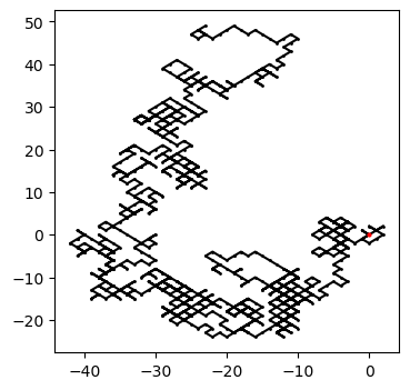
Single Walker Plot
With your working code, plot the walk of a single walker. Here is a code.
i_walker = 10
fig = plt.figure(figsize=(4,4))
ax=fig.add_subplot()
ax.plot(walks[i_walker,:,0], walks[i_walker,:,1], "-o", markersize=1, color="black")
ax.plot(walks[i_walker,0,0], walks[i_walker,0,1], "o", markersize=2, color="red")
[<matplotlib.lines.Line2D at 0x15e7eb890>]
Animation With your working code, you can use the animation script below to create an animation of the random walk output. Note: there are some visual artifacts, related to the fact that the steps are on a grid in increments of 1.
L = np.max(walks)
fig = plt.figure(figsize=(4,4))
ax = fig.add_subplot()
ax.set_xlim(-L,L)
ax.set_ylim(-L,L)
pts, = ax.plot([], [], "o", markersize=1, color = "black", alpha = .5)
plt.close()
def init():
pts.set_data([], [])
return pts,
def draw(i):
x = walks[:,i,0]
y = walks[:,i,1]
pts.set_data(x,y)
return pts,
anim = animation.FuncAnimation(fig, draw, frames=walks.shape[1], interval=50, blit=True)
# Save the animation as a GIF
anim.save('random_walk_animation.gif', writer='pillow', fps=20, dpi=80)
# # Display the saved GIF
# from IPython.display import Image
# Image('random_walk_animation.gif')

matplotlib.rcParams['animation.writer'] = 'ffmpeg'
matplotlib.rcParams['animation.codec'] = 'h264'
#HTML(anim.to_html5_video())
HTML(anim.to_jshtml())