3.1. Arrays in Numpy#
Draft version - do not distribute
3.1.1. NumPy Arrays: The Foundation of Scientific Computing#
NumPy arrays are the foundation of scientific computing in Python. Arrays are the data structure that makes Python a usable tool for data science, machine learning, and numerical analysis (i.e., scientific computing). Without arrays, Python would be impractical as a scientific programming language.
Ultimately, all data has to be represented as numbers. And all data science methods are mathematical manipulations of these numbers. Arrays are the natural—perhaps the only—way to organize data.
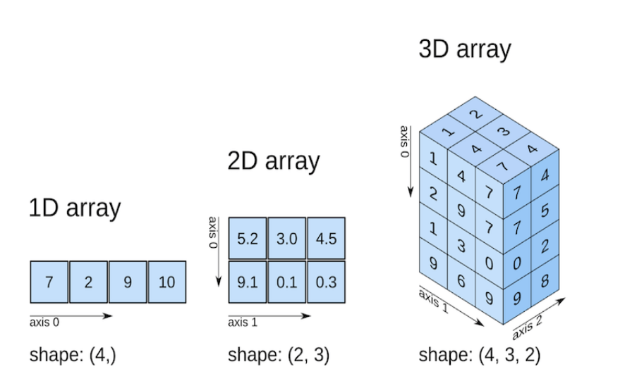
NumPy arrays are multi-dimensional grids of values that can represent vectors, matrices, or higher-dimensional data structures. Each element in an array has a specific location identified by a tuple of integer indices. Python uses zero-based indexing, so the first element is always at index 0.
These arrays are specifically designed and optimized for efficient numerical computation and data manipulation, making them far superior to standard Python lists for mathematical operations. Objects like data frames or dictionaries cannot operate like arrays.
Vectorization allows NumPy to perform operations on entire arrays simultaneously, eliminating the need for explicit loops and dramatically improving performance.
Broadcasting enables mathematical operations between arrays of different shapes through NumPy’s broadcasting rules, providing flexibility in how you combine data.
Understanding NumPy arrays is essential for anyone working in scientific computing with Python. They form the foundation for virtually every major scientific Python library, including pandas, scikit-learn, and matplotlib. You must be able to think in arrays. (Goodbye dataframes, lists, dictionaries, etc.)
3.1.2. Mathematical Notation for Arrays and Matrices#
Real Numbers A real number is any number that can be found on the number line. This includes:
Natural numbers: 1, 2, 3, 4, …
Whole numbers: 0, 1, 2, 3, 4, …
Integers: …, -2, -1, 0, 1, 2, …
Rational numbers: Any number that can be expressed as a fraction (like 1/2, -3/4, or 0.75)
Irrational numbers: Numbers that cannot be expressed as fractions (like π, √2, or e)
Real numbers are called “real” to distinguish them from imaginary numbers or complex numbers.
Any measurement you make in the physical world—length, weight, temperature, time—will be a real number. In this course, we will deal exclusively with real numbers.
The mathematical symbol for the set of real numbers is \(\mathbb{R}\).
3.1.3. Notation for Array and Matrix Dimensions#
Consider the array \(A = [ 1, 3.3, -10, 5.78 ]\). All the elements of \(A\) are real numbers. Additionally, \(A\) has 4 elements. We say that \(A\) is an element of \(\mathbb{R}^4\), an array of size 4 with real elements.
Consider the matrix
The matrix \(B\) has 4 rows and 3 columns, and is composed of real numbers; it is a member of \(\mathbb{R}^{4 \times 3}\).
In general, an array that is a member of \(\mathbb{R}^{n\times m}\) has \(n\) rows and \(m\) columns and \(n\times m\) elements.
Likewise, an array that is a member of \(\mathbb{R}^{n\times m\times l}\) has \(n\) elements along the first dimension, \(m\) elements along the second dimension, \(l\) elements along the third dimension, and \(n\times m\times l\) total elements.
3.1.4. Size, Shape, Indexing, and All That#
Let us consider two arrays, one a vector, the other a matrix.
Note that \(a\) is an member of \(\mathbb{R}^3\) and \(b\) is a memeber of \(\mathbb{R}^{3 \times 3}\).
These two arrays have Python representations written as:
a = np.array([3.0, -2.0, 8.0])
b = np.array([[4.0, 3.0, 1.0], [-2.0, 0, 1.0], [6.0, 10.0, -5.0]])
3.1.5. The Size and Shape of a NumPy Array#
The size of the array is the total number of elements. You can obtain the size by using the attribute array.size. Here is a code snippet example:
print(a.size)
print(b.size)
For our example arrays, \(a\) has size 3, and \(b\) has size 9.
The shape of the array is the number of elements along each dimension of the array. You can obtain the shape by using the attribute array.shape. Here is a code snippet example:
print(a.shape)
print(b.shape)
The attribute shape returns a tuple. The first element of the tuple is the size of the first dimension, the second element is the size of the second dimension, and so on.
import numpy as np

a= np.array([3.0, -2.0, 8.0 ])

b= np.array([[4.0 , 3.0 , 1.0],[ -2.0 , 0 , 1.0],[ 6.0 , 10.0 , -5.0]])

print(a.size)
print(b.size)

print(a.shape)
print(b.shape)
3
9
(3,)
(3, 3)
3.1.6. Indexing#
The elements of an array are marked by an integer called the index. Consider our example, a= np.array([3.0, -2.0, 8.0 ]) .
the 0 element is 3.0
the 1 element is -2.0
the 2 element is 8.0
For our matrix example, the index is two dimensional. The first index marks the row location, while the second index marks the column location. Consider our example,
below is code to loop through each element and display its value.
for i in range(3):
    for j in range(3):
        val = b[i,j]
        print(f"The value at row {i} and column {j} is {val}.")
for i in range(3):
    for j in range(3):
        val = b[i,j]
        print(f"The value at row {i} and column {j} is {val}.")
The value at row 0 and column 0 is 4.0.
The value at row 0 and column 1 is 3.0.
The value at row 0 and column 2 is 1.0.
The value at row 1 and column 0 is -2.0.
The value at row 1 and column 1 is 0.0.
The value at row 1 and column 2 is 1.0.
The value at row 2 and column 0 is 6.0.
The value at row 2 and column 1 is 10.0.
The value at row 2 and column 2 is -5.0.
3.1.6.1. Slicing#
Slicing is the process of extracting a subset of an array.
3.1.6.2. 1D Array Slicing#
Let:
a = np.array([10, 20, 30, 40, 50])
Slice Syntax |
Description |
Output |
|---|---|---|
|
Elements from index 1 to 3 |
|
|
First 3 elements |
|
|
Last 3 elements |
|
|
Every 2nd element |
|
|
Reversed array |
|
|
Single element at index 1 |
|
|
Slice containing one element |
|
3.1.6.3. 2D Array Slicing#
Let:
b = np.array([[1, 2, 3],
              [4, 5, 6],
              [7, 8, 9]])
Slice Syntax |
Description |
Output |
|---|---|---|
|
First row |
|
|
Second column |
|
|
Sub-matrix (2 rows, 2 cols) |
|
|
Reverse rows |
|
|
Reverse columns |
|
|
Center value (row 1, col 1) |
|
3.1.7. Higher Dimensional Arrays#
Higher dimensional arrays are possible but hard to visualize.
Here is an example, using the random.rand function to generate random numbers between 0 and 1:
C = np.random.rand(3, 4, 2)
C=np.random.rand(3,4,2)
C
array([[[0.2143009 , 0.42372487],
        [0.86528373, 0.78714132],
        [0.98448767, 0.64353423],
        [0.91283206, 0.95580231]],

       [[0.60234985, 0.00193377],
        [0.17847898, 0.31635551],
        [0.23757972, 0.90411619],
        [0.3204744 , 0.33974712]],

       [[0.34586156, 0.31888948],
        [0.36626589, 0.41428858],
        [0.07683998, 0.41359096],
        [0.95698906, 0.06891337]]])
C.shape
(3, 4, 2)
3.1.8. Element-Wise Operations#
Element-wise operations apply an operation individually to each element in an array or between matching elements of two arrays. Here are some examples. Let:
a = np.array([1, 2, 3])
b = np.array([4, 5, 6])
Operation |
Code |
Output |
|---|---|---|
Addition |
|
|
Subtraction |
|
|
Multiplication |
|
|
Division |
|
|
Power |
|
|
Scalar Addition |
|
|
Scalar Multiplication |
|
|
Modulo |
|
|
# Import quiz functions
from quiz_indexing_utils import get_all_quizzes
# Import Markdown functions
from IPython.display import Markdown, display

quizzes = get_all_quizzes()
display(Markdown("### Problem 1"))
quizzes[0]
Problem 1
Explanation: Remember that Python uses zero-based indexing. Let's trace through the array:
Value: 12 35 7 89 23 56 41 18 94 67
So arr[6] = 41. The element at index 6 is 41.
display(Markdown("### Problem 2"))
quizzes[1]
Problem 2
Explanation: Using zero-based indexing:
Value: 45 12 78 33 91 27 65 88
So data[3] = 33. The element at index 3 is 33.
display(Markdown("### Problem 3"))
quizzes[2]
Problem 3
Explanation: Negative indexing counts from the end of the array:
Value: 5 15 25 35 45 55
Negative Index: -6 -5 -4 -3 -2 -1
So numbers[-2] = 45. The element at index -2 is the second-to-last element, which is 45.
display(Markdown("### Problem 4"))
quizzes[3]
Problem 4
arr[2:5]?Explanation: Array slicing uses [start:end] where end is exclusive:
Value: 10 20 30 40 50 60 70 80
arr[2:5] selects indices 2, 3, and 4 (index 5 is excluded).
So arr[2:5] = [30, 40, 50].
display(Markdown("### Problem 5"))
quizzes[4]
Problem 5
values[1::3]?Explanation: The slice [1::3] means start at index 1, go to the end, with step 3:
Value: 2 4 6 8 10 12 14 16 18 20
Starting at index 1 (value 4), then every 3rd element:
• Index 1: 4
• Index 4: 10
• Index 7: 16
So values[1::3] = [4, 10, 16].
display(Markdown("### Problem 6"))
quizzes[5]
Problem 6
letters[4:1:-1]?Explanation: The slice [4:1:-1] means start at index 4, go to index 1 (exclusive), with step -1 (reverse):
Value: 'A' 'B' 'C' 'D' 'E' 'F'
Starting at index 4 ('E'), going backwards to index 1 (exclusive):
• Index 4: 'E'
• Index 3: 'D'
• Index 2: 'C'
So letters[4:1:-1] = ['E', 'D', 'C'].
display(Markdown("### Problem 7"))
quizzes[6]
Problem 7
[40, 50, 60],
[70, 80, 90]])
matrix[1, 2]?Explanation: For 2D arrays, indexing works as [row, column] with zero-based indexing:
Row 0: 10 20 30
Row 1: 40 50 60
Row 2: 70 80 90
So matrix[1, 2] means row 1, column 2, which is 60.
display(Markdown("### Problem 8"))
quizzes[7]
Problem 8
[7, 9, 11],
[13, 15, 17]])
grid[2, 0]?Explanation: Using [row, column] indexing with zero-based indexing:
Row 0: 1 3 5
Row 1: 7 9 11
Row 2: 13 15 17
So grid[2, 0] means row 2, column 0, which is 13.
display(Markdown("### Problem 9"))
quizzes[8]
Problem 9
[8, 10, 12],
[14, 16, 18]])
data[-1, -2]?Explanation: Negative indexing works in 2D arrays too:
Col 0 Col 1 Col 2
Row -3/0: 2 4 6
Row -2/1: 8 10 12
Row -1/2: 14 16 18
So data[-1, -2] means last row, second-to-last column, which is 16.
display(Markdown("### Problem 10"))
quizzes[9]
Problem 10
[4, 5, 6],
[7, 8, 9]])
matrix[0:2, 1:3]?Explanation: For 2D slicing, the syntax is [row_slice, column_slice]:
Row 0: 1 2 3
Row 1: 4 5 6
Row 2: 7 8 9
• 0:2 means rows 0 and 1 (row 2 excluded)
• 1:3 means columns 1 and 2 (column 3 excluded)
So we get the intersection: [[2, 3], [5, 6]]
display(Markdown("### Problem 11"))
quizzes[10]
Problem 11
[40, 50, 60],
[70, 80, 90],
[100, 110, 120]])
data[:, 1]?Explanation: The slice [:, 1] means all rows, column 1:
Row 0: 10 20 30
Row 1: 40 50 60
Row 2: 70 80 90
Row 3: 100 110 120
Column 1 contains: [20, 50, 80, 110]
display(Markdown("### Problem 12"))
quizzes[11]
Problem 12
[5, 6, 7, 8],
[9, 10, 11, 12],
[13, 14, 15, 16]])
grid[::2, ::2]?Explanation: The slice [::2, ::2] means every 2nd row and every 2nd column:
Row 0: 1 2 3 4
Row 1: 5 6 7 8
Row 2: 9 10 11 12
Row 3: 13 14 15 16
Selecting rows 0, 2 (every 2nd row) and columns 0, 2 (every 2nd column):
Result: [[1, 3], [9, 11]]
3.1.9. NumPy Array Axes#
Many NumPy operations can be performed on a single dimension of a multidimensional array.
Consider generating a 3 by 4 array of random numbers from 0 to 1.
a = np.random.rand(3,4)
print(a.shape)
You can take the mean of the array as follows:
print(np.mean(a))
You can take the mean along the columns by specifying axis=0; operations down rows correspond to axis 0.
print(np.mean(a, axis=0))
The result is a 4-element array of means along each column.
Likewise, you can take the mean along each row by specifying axis=1; operations across columns correspond to axis 1.
print(np.mean(a, axis=1))
The result is a 3-element array of means along each row.
a = np.random.rand(3,4)
a
array([[0.49890031, 0.16540555, 0.74273468, 0.59559183],
       [0.53641592, 0.70786498, 0.56419282, 0.61503524],
       [0.49892178, 0.97712926, 0.67520771, 0.24520926]])
np.mean(a)
np.float64(0.5685507794865094)
np.mean(a,axis=0)
array([0.51141267, 0.61679993, 0.66071174, 0.48527878])
np.mean(a,axis=1)
array([0.50065809, 0.60587724, 0.599117 ])