6.6. Newton’s Method for Optimization#
Newton’s method can be used to find a local minimum or maximum of a function \(f(x)\). To find the extrema of a function, we replace \(f\) with \(f'\) and \(f'\) with \(f''\) in Newton’s root-finding method. The iteration formula is
Problem
Explain why we replace \(f\) with \(f'\) and \(f'\) with \(f''\) in Newton’s root-finding method when searching for extrema.
Solution
At a local minimum or maximum, the derivative \(f'(x) = 0\). Therefore, finding an extremum is equivalent to finding a root of \(f'(x)\).
Newton’s method for finding a root of a function \(g(x)\) uses the formula
To find where \(f'(x) = 0\), we set \(g(x) = f'(x)\). Then \(g'(x) = f''(x)\), and Newton’s formula becomes
Thus, we are applying Newton’s root-finding method to the derivative \(f'(x)\), which requires us to use the second derivative \(f''(x)\).
The method can be extended to multiple dimensions
where
\(\nabla f(\mathbf{x})\) is the gradient (first derivative)
\(H_f(\mathbf{x})\) is the Hessian matrix (second derivative for multidimensional problems)
The Hessian matrix is
import numpy as np
%matplotlib inline
import matplotlib.pyplot as plt
from mpl_toolkits.mplot3d import Axes3D
from matplotlib import animation
from IPython.display import display, Image
from IPython.display import HTML

from jax import grad, hessian
import jax.numpy as jnp
from functools import partial
---------------------------------------------------------------------------
ModuleNotFoundError                       Traceback (most recent call last)
Cell In[1], line 9
      6 from IPython.display import display, Image
      7 from IPython.display import HTML
----> 9 from jax import grad, hessian
     10 import jax.numpy as jnp
     11 from functools import partial

ModuleNotFoundError: No module named 'jax'
Here is Newton method for root finding code.
def newtons_method(f, x0, max_iter=1000, tol=1e-6, monitor=False):
    """
    Newton's method for optimization using JAX automatic differentiation.

    Parameters
    ----------
    f : callable
        Objective function to minimize
    x0 : array_like
        Initial guess
    max_iter : int
        Maximum number of iterations
    tol : float
        Convergence tolerance
    monitor : bool
        If True, return history of function values

    Returns
    -------
    x_min : ndarray
        Estimated minimum point
    loss : list (optional)
        History of function values if monitor=True
    """
    x = jnp.array(x0, dtype=float)

    # Gradient and Hessian functions via JAX
    df = grad(f)
    ddf = hessian(f)

    if monitor:
        loss = [f(x)]

    # Newton's method loop
    for i in range(max_iter):
        # Evaluate gradient and Hessian
        grad_val = df(x)
        hess_val = ddf(x)

        # Newton's update: solve H*delta = -grad for delta
        delta_x = jnp.linalg.solve(hess_val, -grad_val)
        x_new = x + delta_x

        if monitor:
            loss.append(f(x_new))

        # Check convergence
        if jnp.linalg.norm(delta_x) < tol:
            print(f"Converged in {i+1} iterations")
            if monitor:
                return x_new, loss
            else:
                return x_new

        x = x_new

    print(f"Did not converge within {max_iter} iterations")

    if monitor:
        return x, loss
    else:
        return x
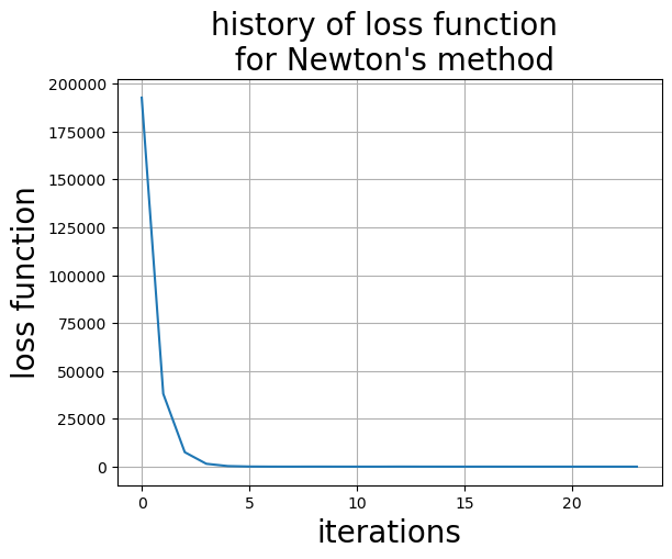
Example: Solving a Nonlinear System Using Least Squares
Consider finding the solution to the nonlinear system, a function I got from Wikipedia,
We can solve this using Newton’s optimization method by minimizing the objective function
where \(\mathbf{F} = [f_0, f_1, f_2]^T\).
Minimizing \(g(\mathbf{x})\) is equivalent to minimizing the squared norm \(\|\mathbf{F}\|^2\).
def wiki_func(z):
    x0, x1, x2 = z

    f0=3*x0 - jnp.cos(x1*x2) - 3/2
    f1=4*x0**2 - 625*x1**2 + 2*x1 - 1
    f2=jnp.exp(-x0*x1) + 20*x2 + (10*jnp.pi-3)/3

    return jnp.array([f0, f1, f2])

def objective(z):

    f=wiki_func(z)

    return jnp.dot(f,f)/2.0
x, loss_newton=newtons_method(objective, jnp.ones(3), monitor=True)
print("Solution and objective", x, objective(x))
Converged in 23 iterations
Solution and objective [ 0.8331966   0.05494366 -0.5213615 ] 7.1054274e-15
# check solution
wiki_func(x)
Array([0.0000000e+00, 1.1920929e-07, 0.0000000e+00], dtype=float32)
ax=plt.subplot()
ax.set_title("history of loss function \n for Newton's method", size=20)
ax.set_xlabel("iterations", size=20)
ax.set_ylabel("loss function", size=20)
ax.plot(loss_newton)
ax.grid()
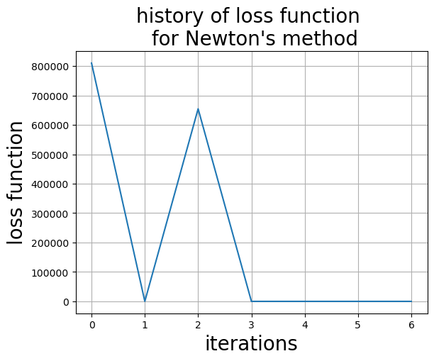
Example Minimize the Rosenbrock function
which has a minima at \((x,y)=(1,1)\). How does Newton’s method do?
def rosenbrock(X):
    # minima at 1,1
    x, y = X
    return (1 - x)**2 + 100 * (y - x**2)**2
x, loss_newton=newtons_method(rosenbrock, jnp.ones(2)*10, monitor=True)
print("Solution and objective", x, rosenbrock(x))
Converged in 6 iterations
Solution and objective [1. 1.] 0.0
ax=plt.subplot()
ax.set_title("history of loss function \n for Newton's method", size=20)
ax.set_xlabel("iterations", size=20)
ax.set_ylabel("loss function", size=20)
ax.plot(loss_newton)
ax.grid()
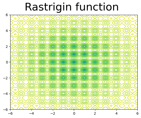
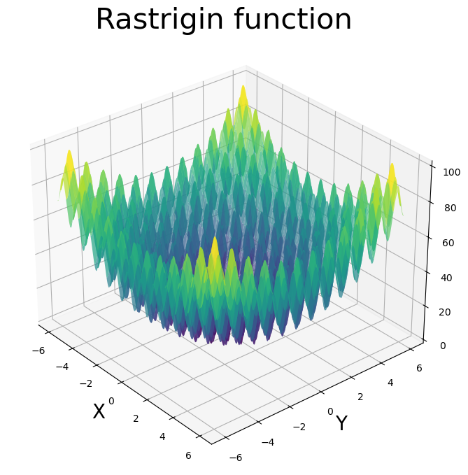
Example Try Newton’s method on the Rastrigin function. The Rastrigin function is non-convex and has many local minima, with a global minima at \((x,y)=(0,0)\).
def rastrigin(X):
    #minima at 0, 0
    # many local minima
    x, y = X
    return 20 + x**2 + y**2 - 10 * (jnp.cos(2 * jnp.pi * x) + jnp.cos(2 * jnp.pi * y))
x=np.linspace(-6,6,1000)
y=np.linspace(-6,6,1000)

fig=plt.figure()
fig.suptitle("Rastrigin function", size=30)
ax=fig.add_subplot()

X,Y=np.meshgrid(x,y)
Z=rastrigin([X,Y])
ax.contour(X,Y,np.log(Z), levels=50)
<matplotlib.contour.QuadContourSet at 0x15c9d7e00>
X, Y = np.meshgrid(x, y)

Z = rastrigin([X,Y])

# Create the figure and axes object
fig = plt.figure(figsize=(8, 10))
ax = fig.add_subplot(111, projection='3d')

# Plot the surface
ax.plot_surface(X, Y, Z, cmap='viridis', alpha=.7)

# Set labels and title
ax.set_xlabel('X', size=20)
ax.set_ylabel('Y', size=20)
ax.set_title('Rastrigin function', size=30 )
ax.view_init(azim=-40)
x, loss_newton=newtons_method(rastrigin, jnp.ones(2)*5, tol=1e-10,monitor=True)
print("Solution and objective", x, rastrigin(x))
Did not converge within 1000 iterations
Solution and objective [4.9746914 4.9746914] 49.747444
ax=plt.subplot()
ax.set_title("history of loss function \n for Newton's method", size=20)
ax.set_xlabel("iterations", size=20)
ax.set_ylabel("loss function", size=20)
ax.plot(loss_newton, "-o")
ax.grid()
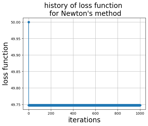
Question How did Newton’s method perform on the Rastrigin function? Did it find the global minima? Explain what happened. Can you think of anything you could do to help improve the result?