6.2. Convex Functions and Optimization

For a convex function, any local minimum is also a global minimum. Optimization with convex functions is often well-behaved, as a global minimum is guaranteed. So, what is a convex function? I would say it is something akin to a bowl with no large ripples (local minima)—it is a nice smooth ride to the bottom. But that is not good enough; we need a mathematical definition.

A function \(f: \mathbb{R}^n \to \mathbb{R}\) is convex if for all points \(\mathbf{x}, \mathbf{y}\) in its domain and for all \(\lambda \in [0, 1]\), the following inequality holds:

(6.36)\[\begin{equation} f(\lambda \mathbf{x} + (1-\lambda)\mathbf{y}) \leq \lambda f(\mathbf{x}) + (1-\lambda)f(\mathbf{y}). \end{equation}\]

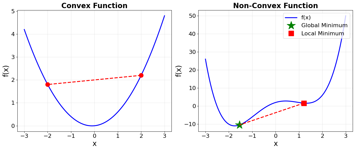
The geometric interpretation is as follows. The left side represents the function value at a point on the line segment connecting \(\mathbf{x}\) and \(\mathbf{y}\), while the right side represents the corresponding point on the line segment connecting \((\mathbf{x}, f(\mathbf{x}))\) and \((\mathbf{y}, f(\mathbf{y}))\) on the graph. Therefore, a function is convex if and only if the line segment (called the secant line) connecting any two points on its graph lies on or above the graph itself. Below is a plot exemplifying convexity. The left panel shows a convex function, while the right panel shows a non-convex function.

import numpy as np
import matplotlib.pyplot as plt

# Create figure
fig, axes = plt.subplots(1, 2, figsize=(14, 6))

# ========== LEFT PANEL: CONVEX FUNCTION ==========
ax = axes[0]

# Define convex function
x = np.linspace(-3, 3, 500)
y = 0.5 * x**2 + 0.1 * x

# Plot the function
ax.plot(x, y, 'b-', linewidth=2.5, label='f(x)')

# Choose two points for the secant line
x1, x2 = -2, 2
y1 = 0.5 * x1**2 + 0.1 * x1
y2 = 0.5 * x2**2 + 0.1 * x2

# Create points along the line segment
lambdas = np.linspace(0, 1, 100)
x_line = lambdas * x1 + (1 - lambdas) * x2
y_secant = lambdas * y1 + (1 - lambdas) * y2
y_func = 0.5 * x_line**2 + 0.1 * x_line

# Plot the secant line
ax.plot(x_line, y_secant, 'r--', linewidth=2.5)

# Mark the endpoints
ax.plot([x1, x2], [y1, y2], 'ro', markersize=12)

# # Shade the region showing secant ≥ function
# ax.fill_between(x_line, y_func, y_secant, alpha=0.3, color='green',
#                 label='Secant ≥ Function')

ax.set_xlabel('x', fontsize=20)
ax.set_ylabel('f(x)', fontsize=20)
ax.set_title('Convex Function', fontsize=20, fontweight='bold')
ax.grid(True, alpha=0.3)
ax.tick_params(labelsize=16)

# ========== RIGHT PANEL: NON-CONVEX FUNCTION ==========
ax = axes[1]

# Define non-convex function with local and global minima
x = np.linspace(-3, 3, 500)
y = x**4 - 5*x**2 + 4*x + 2

# Plot the function
ax.plot(x, y, 'b-', linewidth=2.5, label='f(x)')

# Global minimum around x ≈ -1.54
x_global = -1.54
y_global = x_global**4 - 5*x_global**2 + 4*x_global + 2

# Local minimum around x ≈ 1.21
x_local = 1.21
y_local = x_local**4 - 5*x_local**2 + 4*x_local + 2


# Create points along the line segment
lambdas = np.linspace(0, 1, 100)
x_line = lambdas * x_global + (1 - lambdas) * x_local


y_secant = lambdas * y_global + (1 - lambdas) * y_local

# Plot the minima
ax.plot(x_global, y_global, 'g*', markersize=25, label='Global Minimum')
ax.plot(x_local, y_local, 'rs', markersize=15, label='Local Minimum')
ax.plot(x_line, y_secant, 'r--', linewidth=2.5)

ax.set_xlabel('x', fontsize=20)
ax.set_ylabel('f(x)', fontsize=20)
ax.set_title('Non-Convex Function', fontsize=20, fontweight='bold')
ax.legend(fontsize=16, loc='upper right')
ax.grid(True, alpha=0.3)
ax.tick_params(labelsize=16)

plt.tight_layout()
plt.savefig('convex_vs_nonconvex.png', dpi=150, bbox_inches='tight')
plt.show()

For twice-differentiable functions, convexity can be characterized using derivatives. In single variable calculus, if \(\frac{d^2 f}{dx^2} \geq 0\) for all \(x\), then the function is convex. This generalizes to multivariable functions through the Hessian matrix. The function \(f\) is convex if and only if its Hessian matrix \(H(\mathbf{x})\) is positive semi-definite for all \(\mathbf{x}\) in the domain.

To check convexity, we examine the eigenvalues of the Hessian. Since the Hessian is symmetric, it has real eigenvalues. The Hessian is positive semi-definite if and only if all eigenvalues are non-negative (\(\lambda_i \geq 0\)). If all eigenvalues are strictly positive (\(\lambda_i > 0\)), the Hessian is positive definite, corresponding to strict convexity.

Many models in machine learning are convex. Linear regression with squared loss is convex because the objective function \(||\mathbf{y} - X\mathbf{\beta}||^2\) is a quadratic function with a positive semi-definite Hessian. Logistic regression with log loss is also convex (we showed this in the logistic regression notebook). However, deep neural networks are non-convex due to the composition of nonlinear activation functions, which can make training them difficult.