6.1. Introduction to Fourier Analysis#
You can have a look at the Wikipedia article on Fourier analysis to get a comprehensive overview of the subject. The simplest way to summarize Fourier analysis (from my perspective) is as the study of how functions can be represented by oscillating functions, such as cosines, sines, and complex exponentials.
You may already be familiar with the Fourier series, which represents a periodic function as a discrete summation of cosines, sines, or complex exponentials. The continuous Fourier transform extends the concept of the Fourier series beyond a single periodic interval to the entire real number line, mapping the function across a continuous continuum of frequencies.
The discrete Fourier transform (DFT) is the analogue of the Fourier transform applied to discrete, finite sequence data (for me conceptually sharing much in common with the Fourier series). The fast Fourier transform (FFT) is the algorithm used to compute the DFT efficiently on a computer. The FFT algorithm evaluates the DFT in \(\mathcal{O}(N \log N)\) operations, which represents a dramatic improvement in computational efficiency compared to a naive matrix-vector implementation requiring \(\mathcal{O}(N^2)\) operations.
To start, we need to establish some essential nomenclature regarding periodic and oscillating functions.
A periodic function is a function that repeats its behavior at regular intervals of space or time. For example, the hour hand of a clock is periodic in time, completing a full cycle every 12 hours. Similarly, if an athlete runs around a standard 400-meter track at a constant speed of 10 meters per second, each lap requires 40 seconds. By continuing this lap running indefinitely, the motion becomes a periodic function with a period of 40 seconds because the runner returns to the exact same position on the track at every 40-second interval.
For functions that are periodic in time, the period \(T\) represents the duration required for the function to complete one full cycle, which satisfies the relationship
In this temporal context, the variable \(t\) represents time and can be measured in units such as seconds, hours, days, or years.
For functions that are periodic in space, the wavelength \(\lambda\) represents the spatial distance required for the function to repeat itself, satisfying the condition
Here, the variable \(x\) represents spatial position, typically measured in meters, yards, feet, or inches.
For a time-dependent function, the frequency \(f\) characterizes the number of complete cycles or revolutions executed per unit of time. In physics, time is most frequently quantified in seconds, meaning that frequency reflects the number of cycles per second, a quantity measured in Hertz [Hz].
Frequency and period are inversely related by the equation \(f = 1/T\). Returning to the track example, a runner completing a lap every 40 seconds has a period of \(T = 40\text{ s}\) and a corresponding frequency of \(f = 1/40\text{ Hz}\).
6.1.1. Example Problem#
An ocean buoy sits in open water and records the passing of surface waves. The buoy bobbing up and down completes exactly 15 full vertical oscillations in one minute. What is the period and the frequency of this periodic motion in standard SI units?
Click here to reveal the solution
The frequency represents the number of complete cycles per second. We are given 15 cycles in one minute, and since one minute contains 60 seconds, the frequency is calculated as $\(f = \frac{15\text{ cycles}}{60\text{ s}} = 0.25\text{ Hz}.\)$
Because the period \(T\) is the inverse of the frequency, we find the time required for a single wave cycle to pass is $\(T = \frac{1}{f} = \frac{1}{0.25\text{ Hz}} = 4.0\text{ s}.\)$
The passing ocean waves cause the buoy to repeat its vertical motion every 4.0 seconds.
The trigonometric functions \(\cos(\theta)\) and \(\sin(\theta)\) accept angles as arguments and naturally repeat their values whenever an integer multiple of \(2\pi\) radians is added to the angle, satisfying the conditions
where \(n = 0, 1, 2, \dots\).
The angular frequency \(\omega\) represents the frequency scaled by a factor of \(2\pi\), defined by the relationship
When analyzing time-dependent oscillations, we express the time-varying angle as \(\theta = \omega t\).
The animation below displays the trajectory of a particle moving along the unit circle for two distinct values of \(\omega\). The trajectory associated with the larger angular frequency progresses at a visibly faster rate than the one with the lower angular frequency. To visualize the trigonometric components, the animation includes the adjacent and opposite legs of the reference triangle, which explicitly track the instantaneous values of \(\cos(\omega t)\) and \(\sin(\omega t)\) along the axes.
import numpy as np
import matplotlib.pyplot as plt
from matplotlib.animation import FuncAnimation
from IPython.display import HTML

# Define angular frequencies (e.g., omega_1 = 1 rad/s, omega_2 = 2.5 rad/s)
omega1 = 1.0
omega2 = 2.5

# Set up time array for a smooth animation
t_max = 2 * np.pi / omega1
fps = 30
frames = 120
t_eval = np.linspace(0, t_max, frames)

# Set up the figure for side-by-side plots
fig, (ax1, ax2) = plt.subplots(1, 2, figsize=(10, 5))
theta_fill = np.linspace(0, 2 * np.pi, 100)

for ax in (ax1, ax2):
    ax.plot(np.cos(theta_fill), np.sin(theta_fill), color='gray', linestyle='--', alpha=0.5)
    ax.axhline(0, color='black', linewidth=0.5)
    ax.axvline(0, color='black', linewidth=0.5)
    ax.set_xlim(-1.2, 1.2)
    ax.set_ylim(-1.2, 1.2)
    ax.set_aspect('equal')
    ax.grid(True, which='both', linestyle=':', alpha=0.5)

ax1.set_title(rf"$\omega_1 = {omega1}$ rad/s (Slower)")
ax2.set_title(rf"$\omega_2 = {omega2}$ rad/s (Faster)")

# Initialize graphic elements for Axis 1
line_hyp1, = ax1.plot([], [], color='black', linewidth=1.5)
line_adj1, = ax1.plot([], [], color='crimson', linewidth=2, label=r'$\cos(\omega t)$')
line_opp1, = ax1.plot([], [], color='royalblue', linewidth=2, label=r'$\sin(\omega t)$')
dot1, = ax1.plot([], [], 'ko', markersize=8)

# Initialize graphic elements for Axis 2
line_hyp2, = ax2.plot([], [], color='black', linewidth=1.5)
line_adj2, = ax2.plot([], [], color='crimson', linewidth=2, label=r'$\cos(\omega t)$')
line_opp2, = ax2.plot([], [], color='royalblue', linewidth=2, label=r'$\sin(\omega t)$')
dot2, = ax2.plot([], [], 'ko', markersize=8)

ax1.legend(loc='upper left')
ax2.legend(loc='upper left')

def update(frame):
    t = t_eval[frame]

    # Subplot 1 update
    x1, y1 = np.cos(omega1 * t), np.sin(omega1 * t)
    line_hyp1.set_data([0, x1], [0, y1])
    line_adj1.set_data([0, x1], [0, 0])
    line_opp1.set_data([x1, x1], [0, y1])
    dot1.set_data([x1], [y1])

    # Subplot 2 update
    x2, y2 = np.cos(omega2 * t), np.sin(omega2 * t)
    line_hyp2.set_data([0, x2], [0, y2])
    line_adj2.set_data([0, x2], [0, 0])
    line_opp2.set_data([x2, x2], [0, y2])
    dot2.set_data([x2], [y2])

    return line_hyp1, line_adj1, line_opp1, dot1, line_hyp2, line_adj2, line_opp2, dot2

ani = FuncAnimation(fig, update, frames=frames, interval=1000/fps, blit=True)
plt.close()

# To view inside Jupyter, render as HTML5 video:
HTML(ani.to_html5_video())
We can link complex exponentials to cosines and sines via Euler’s formula, which states that
This profound identity maps a complex number of unit magnitude to a specific position on the complex plane, where the real part corresponds to the horizontal cosine projection and the imaginary part corresponds to the vertical sine projection.
6.1.1.1. Example: Evaluating a Negative Angle#
Use Euler’s formula to evaluate \(e^{-i\theta}\) and express the final result in terms of \(\cos(\theta)\) and \(\sin(\theta)\).
Click here to reveal the solution
Applying Euler’s formula directly with a negative argument yields $\(e^{i(-\theta)} = \cos(-\theta) + i \sin(-\theta).\)$
Because the cosine function is even, \(\cos(-\theta) = \cos(\theta)\). Conversely, because the sine function is odd, \(\sin(-\theta) = -\sin(\theta)\). Substituting these parity relationships back into the expression gives the identity $\(e^{-i\theta} = \cos(\theta) - i \sin(\theta).\)$
6.1.1.2. Example: Isolating Trigonometric Functions#
Using the expressions for \(e^{i\theta}\) and \(e^{-i\theta}\), derive an explicit formula for \(\cos(\theta)\) purely in terms of complex exponentials.
Click here to reveal the solution
We begin with the standard Euler formula and the result from Problem 1:
Adding these two equations together eliminates the imaginary sine terms on the right side, giving $\(e^{i\theta} + e^{-i\theta} = 2\cos(\theta).\)$
Dividing both sides by 2 isolates the cosine function, yielding the standard exponential definition $\(\cos(\theta) = \frac{e^{i\theta} + e^{-i\theta}}{2}.\)$
6.1.1.3. Problem 3: Complex Magnitude#
Prove that the complex magnitude \(|e^{i\theta}|\) equals 1 for any real value of \(\theta\).
Click here to reveal the solution
The magnitude of any complex number \(z = a + ib\) is defined by the relationship \(|z| = \sqrt{a^2 + b^2}\). Expanding \(e^{i\theta}\) into its real and imaginary parts using Euler’s formula provides \(a = \cos(\theta)\) and \(b = \sin(\theta)\).
Calculating the magnitude then yields $\(|e^{i\theta}| = \sqrt{\cos^2(\theta) + \sin^2(\theta)}.\)$
By the fundamental Pythagorean trigonometric identity, \(\cos^2(\theta) + \sin^2(\theta) = 1\) for all real numbers, simplifying our expression to $\(|e^{i\theta}| = \sqrt{1} = 1.\)$
This confirms that the complex exponential \(e^{i\theta}\) always traces out a path along the perimeter of the unit circle in the complex plane. </details.
6.1.2. The Discrete Fourier Transform (DFT)#
Every time you stream a song on Spotify, talk to a voice assistant on your smartphone, or switch on active noise-canceling headphones, you are relying on the Discrete Fourier Transform. In industry, raw data almost always arrives as a sequence of measurements changing over time, such as a changing voltage from a microphone or an acceleration reading from an iPhone sensor. While our human ears easily pick out individual pitches, instruments, or voices in a room, a computer only sees a list of numbers representing the signal’s amplitude over time. The DFT is the mathematical prism that splits that single, complicated time-domain signal into its individual frequency components.
6.1.2.1. Defining the Sampled Signal#
Imagine a time-dependent signal \(f(t)\) that has been captured at evenly spaced instances in time, yielding a collection of data points where each digital sample is given by \(f_n = f(t_n)\). The specific timestamps for these samples follow the progression
where \(n = 0, 1, 2, \ldots, N-1\). In this notation, \(t_0\) represents the starting time, \(\Delta t\) represents the constant time step between consecutive measurements (the sampling interval), and \(N\) represents the total number of data points collected.
6.1.2.2. The Transformation Equations#
The Discrete Fourier Transform converts this finite sequence of time-domain samples into a sequence of complex numbers representing the signal in the frequency domain. The forward transformation is defined by the expression
for each frequency index \(m = 0, 1, \ldots, N-1\). Each resulting coefficient \(F_m\) is a complex number that encapsulates both the amplitude (volume) and the phase (timing shift) of a specific sinusoidal component present within the aggregate signal. I will often refer to \(F_m\) as the DFT.
If we know the frequency coefficients, we can perfectly reconstruct our original time-domain samples. This reverse process is governed by the Inverse Discrete Fourier Transform (IDFT), which is given by
The frequencies \(freq_m\) associated with each index \(m\) are linked to the physical sampling interval \(\Delta t\) by the equation
where the indices scale sequentially from \(m = 0\) up to \(m = N-1\). Low values of \(m\) correspond to slow, oscillations, while higher values track rapid, fluctuations.
To build some intuition for the DFT, let us construct a DFT from scratch. We will compare our results to the NumPy implementation. Below is the code.
import numpy as np

# Set random seed for reproducibility
np.random.seed(42)

# Generate sample signal
N = 5
f = np.random.randint(0, 10, size=N)
print("f:", f)


def dft(f):
    """Compute the Discrete Fourier Transform (DFT) via double loop."""
    N = f.size
    F = np.zeros(N, dtype=complex)

    for m in range(N):
        for n in range(N):
            F[m] += np.exp(-2j * np.pi * m * n / N) * f[n]

    return F


def idft(F):
    """Compute the Inverse Discrete Fourier Transform (IDFT) via double loop."""
    N = F.size
    f_rec = np.zeros(N, dtype=complex)

    for m in range(N):
        for n in range(N):
            f_rec[m] += np.exp(2j * np.pi * m * n / N) * F[n]

    return f_rec / N


# Alternative vectorized DFT matrix construction (still O(N^2), but fast in NumPy)
def dft_matrix(f):
    N = f.size
    m = np.arange(N).reshape(-1, 1)
    n = np.arange(N).reshape(1, -1)
    W = np.exp(-2j * np.pi * m * n / N)
    return W @ f


# Compute DFTs
F = dft(f)
F_numpy = np.fft.fft(f)

print("\n--- Forward Transform ---")
print("F (Custom DFT):   ", F)
print("F (NumPy FFT):    ", F_numpy)
print("Close to NumPy?:  ", np.allclose(F, F_numpy))

# Compute Inverse DFTs
f_rec = idft(F)
f_rec_numpy = np.fft.ifft(F_numpy)

print("\n--- Inverse Transform (Round Trip) ---")
print("Round trip (Custom IDFT): ", f_rec)
print("Round trip (NumPy IFFT):  ", f_rec_numpy)
print("Reconstruction matches?:  ", np.allclose(f, f_rec))
f: [6 3 7 4 6]

--- Forward Transform ---
F (Custom DFT):    [26.        +0.j         -0.11803399+1.08981379j  2.11803399+4.61652531j
  2.11803399-4.61652531j -0.11803399-1.08981379j]
F (NumPy FFT):     [26.        +0.j         -0.11803399+1.08981379j  2.11803399+4.61652531j
  2.11803399-4.61652531j -0.11803399-1.08981379j]
Close to NumPy?:   True

--- Inverse Transform (Round Trip) ---
Round trip (Custom IDFT):  [6.-1.42108547e-15j 3.-4.16333634e-16j 7.+1.33226763e-16j
 4.+1.55431223e-16j 6.+1.15463195e-15j]
Round trip (NumPy IFFT):   [6.+0.j 3.+0.j 7.+0.j 4.+0.j 6.+0.j]
Reconstruction matches?:   True
6.1.3. Power Spectral Density (PSD)#
The power spectral density (PSD) measures the power distribution of a signal across its discrete frequency components. It is defined as the square of the magnitude of the DFT coefficients \(F_m\) divided by the square of the total number of data points \(N^2\), giving $\(\text{PSD}_m = \frac{F_m F_m^*}{N^2} = \frac{\vert{}F_m\vert{}^2}{N^2}\)\( where \)F_m^*\( denotes the complex conjugate of \)F_m$.
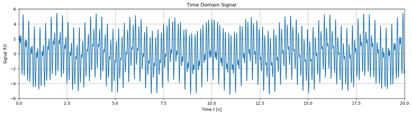
To demonstrate how the power spectral density, we construct a synthetic temporal signal composed of known frequencies. We evaluate its discrete Fourier transform using NumPy’s FFT algorithm and compute the corresponding PSD.
Consider the time-series signal defined by
where \(t \in [0, T]\) with a total duration \(T = 20\text{ s}\), and the fundamental angular frequency is given by \(\omega_1 = 2\pi / T\). The angular frequencies in the signal correspond to integer harmonics \(\omega_m = m \omega_1\) for mode indices \(m \in \{10, 137, 206\}\).
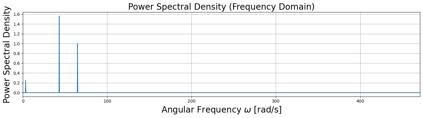
Evaluating the PSD of \(f(t)\) yields three distinct spectral peaks located precisely at these angular frequencies:
\(\omega_{10} = \pi\text{ rad/s} \approx 3.14\text{ rad/s}\) with a relative peak power proportional to \(1^2 / 4 = 0.25\)
\(\omega_{137} = 13.7\pi\text{ rad/s} \approx 43.04\text{ rad/s}\) with a relative peak power proportional to \((-2.5)^2 / 4 = 1.5625\)
\(\omega_{206} = 20.6\pi\text{ rad/s} \approx 64.72\text{ rad/s}\) with a relative peak power proportional to \(2^2 / 4 = 1.0\)
Because \(f(t)\) is real-valued, its Fourier spectrum possesses Hermitian symmetry, meaning \(F_{-m} = F_m^*\). Consequently, the total power of each sinusoid is split equally between its positive and negative frequency components \(+\omega_m\) and \(-\omega_m\). Plotting the PSD against positive frequencies \(\omega \ge 0\) cleanly recovers the constituent modes and their relative power contributions.
import matplotlib.pyplot as plt

# Total time duration (seconds) and fundamental angular frequency
T = 20
omega1 = 2 * np.pi / T

# Harmonic angular frequencies
omega10 = 10 * omega1
omega137 = 137 * omega1
omega206 = 206 * omega1

# Time grid discretization
nt = 3000
t = np.linspace(0, T, nt, endpoint=False)
dt = t[1] - t[0]

# Synthetic time-series signal
f = np.cos(omega10 * t) - 2.5 * np.cos(omega137 * t) + 2 * np.sin(omega206 * t)

# Plot Signal in Time Domain
fig = plt.figure(figsize=(14, 4))
ax = fig.add_subplot()
ax.plot(t, f)
ax.set_xlim(0, T)
ax.set_xlabel("Time $t$ [s]")
ax.set_ylabel("Signal $f(t)$")
ax.set_title("Time Domain Signal")
ax.grid(True)
plt.tight_layout()
plt.show()

# Compute FFT and Frequency Axes
F = np.fft.fft(f)
m = np.fft.fftfreq(f.size) * f.size  # Discrete mode indices

omega = (2 * np.pi / T) * m  # Angular frequency [rad/s]
nu = omega / (2 * np.pi)  # Linear frequency [Hz] (equivalent to m / T)

# Power Spectral Density (|F|^2 / N^2)
PSD = (np.abs(F) / f.size) ** 2

# Plot PSD in Frequency Domain (Positive Frequencies)
fig = plt.figure(figsize=(14, 4))
ax = fig.add_subplot()

# Limit x-axis to positive Nyquist frequency range
ax.plot(omega, PSD)
ax.set_xlim(0, np.max(omega))
ax.set_xlabel(r"Angular Frequency $\omega$ [rad/s]", size=20)
ax.set_ylabel("Power Spectral Density", size=20)
ax.set_title("Power Spectral Density (Frequency Domain)", size=20)
ax.grid(True)

plt.tight_layout()
plt.show()
6.1.3.1. A Simple DFT Noise Filter#
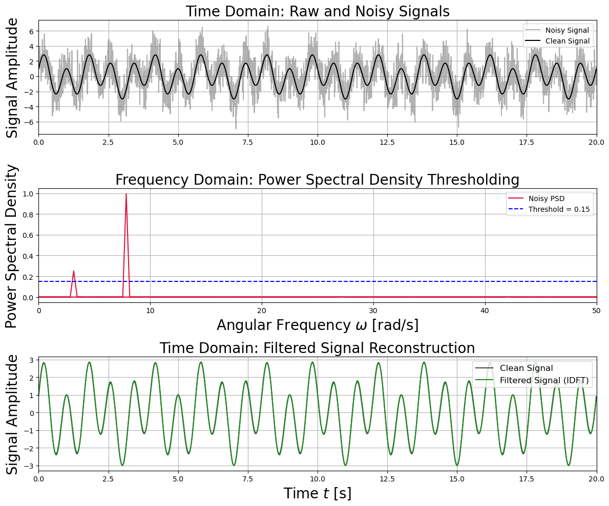
As another demonstration of the discrete Fourier transform, we construct a basic frequency-domain noise filter. While this thresholding approach should not be used for professional settings, it does illustrates the utility of the DFT.
We generate a clean multi-tone signal and contaminate it with additive zero-mean Gaussian noise. Taking the DFT of the noisy signal and evaluating its power spectral density allows us to visually identify signal modes above the background noise floor. By setting a power threshold, we zero out all frequency components falling below this cutoff, effectively suppressing the noise. Finally, applying the inverse DFT (IDFT) reconstructs the filtered signal in the time domain.
# Set random seed for reproducible noise generation
np.random.seed(42)

# --- 1. Signal Generation ---
T = 20.0  # Total time duration [s]
omega1 = 2 * np.pi / T  # Fundamental angular frequency

nt = 3000
t = np.linspace(0, T, nt, endpoint=False)

# Clean signal: combination of low-frequency components
f_clean = np.cos(10 * omega1 * t) + 2.0 * np.sin(25 * omega1 * t)

# Add Gaussian white noise (zero mean, std dev = 1.5)
noise = np.random.normal(0, 1.5, size=nt)
f_noisy = f_clean + noise

# --- 2. Discrete Fourier Transform & PSD ---
F_noisy = np.fft.fft(f_noisy)
m = np.fft.fftfreq(nt) * nt
omega = omega1 * m  # Angular frequency axis

PSD = (np.abs(F_noisy) / nt) ** 2

# --- 3. Frequency Thresholding (Filtering) ---
# Inspect PSD floor and establish a threshold to isolate signal peaks
threshold = 0.15
mask = PSD > threshold

# Zero out frequencies below the power threshold
F_filtered = F_noisy * mask

# --- 4. Reconstruction via Inverse DFT ---
f_filtered = np.real(np.fft.ifft(F_filtered))

# --- 5. Visualization ---
fig, axes = plt.subplots(3, 1, figsize=(12, 10), sharex=False)

# Time Domain: Clean vs. Noisy
axes[0].plot(t, f_noisy, color="gray", alpha=0.6, label="Noisy Signal")
axes[0].plot(t, f_clean, color="black", linewidth=1.5, label="Clean Signal")
axes[0].set_xlim(0, T)
axes[0].set_ylabel("Signal Amplitude",  size=20)
axes[0].set_title("Time Domain: Raw and Noisy Signals",  size=20)
axes[0].legend(loc="upper right")
axes[0].grid(True)

# Frequency Domain: PSD and Threshold
axes[1].plot(omega, PSD, color="crimson", label="Noisy PSD")
axes[1].axhline(
    threshold,
    color="blue",
    linestyle="--",
    linewidth=1.5,
    label=f"Threshold = {threshold}",
)
axes[1].set_xlim(0, 50)  # Focus on positive lower-frequency range
axes[1].set_xlabel(r"Angular Frequency $\omega$ [rad/s]",  size=20)
axes[1].set_ylabel("Power Spectral Density",  size=20)
axes[1].set_title("Frequency Domain: Power Spectral Density Thresholding",  size=20)
axes[1].legend(loc="upper right")
axes[1].grid(True)

# Time Domain: Reconstructed Filtered Signal vs. Clean
axes[2].plot(t, f_clean, color="black", alpha=0.7, label="Clean Signal")
axes[2].plot(
    t,
    f_filtered,
    color="forestgreen",
    linewidth=1.5,
    label="Filtered Signal (IDFT)",
)
axes[2].set_xlim(0, T)
axes[2].set_xlabel("Time $t$ [s]",  size=20)
axes[2].set_ylabel("Signal Amplitude",  size=20)
axes[2].set_title("Time Domain: Filtered Signal Reconstruction",  size=20)
axes[2].legend(loc="upper right", fontsize="large")
axes[2].grid(True)

plt.tight_layout()
plt.show()