8.11. Gradient Descent with Momentum

8.11.1. Momentum

Momentum is an adjustment to the vanilla gradient descent method that serves two purposes. First, it can speed up convergence when the optimizer becomes trapped in a region of large curvature that runs transverse to the optimization direction. I like to imagine this as a riverbed valley: the loss function flows slowly downstream toward the minimum, while the steep valley walls on either side represent regions of large gradient. The optimizer, caught between these walls, bounces back and forth across the valley when it should be moving downstream.

Second, momentum helps the optimizer push through shallow local minima, allowing it to continue toward a lower region of the loss surface.

As a physicist, I have to say, I don’t think gradient descent with momentum has much to do with actual momentum.

I’ll now try to give an intuitive understanding of how the momentum method works; this is my own way of explaining it, hopefully it helps.

To understand momentum, we first need to recognize that the gradient carries directional information.

Consider the function

(8.84)\[\begin{equation} f(x, y) = \frac{1}{4}x^2 + 4y^2 . \end{equation} \]

This function is quadratic in both \(x\) and \(y\), but the curvature in the \(y\) direction is much greater than in the \(x\) direction. The gradient is

(8.85)\[\begin{equation} \nabla f = \begin{bmatrix} \frac{1}{2}x \\[4pt] 8y \end{bmatrix} . \end{equation} \]

Evaluating the gradient at the point \((4, 1)\) gives

(8.86)\[\begin{equation} \nabla f(4,1) = \begin{bmatrix} 2 \\[4pt] 8 \end{bmatrix} , \end{equation} \]

showing that the gradient is larger in the \(y\) direction than in the \(x\) direction at this point.

---

The momentum method uses past gradient evaluations to reduce motion in unwanted directions and accelerate motion in desired ones.

Let’s return to the river valley analogy. The valley walls are steep and therefore have large gradients. The minimum lies downstream, where the river flows slowly, meaning the gradients in that direction are small. Because the optimizer responds strongly to large gradients, it tends to oscillate back and forth between the valley walls instead of moving smoothly downstream. That oscillation is wasted optimization effort—we want to move downstream, not sideways.

To fix this, suppose we combine the gradients from step \(n\) and step \(n-1\). Let’s call the river-valley loss function \(\Phi\). Then, schematically,

(8.87)\[\begin{equation} \begin{split} \nabla \Phi\big|_n + \nabla \Phi\big|_{n-1} &= \begin{bmatrix} \text{gradient downstream} \\[4pt] \text{gradient across valley (say, to the right)} \end{bmatrix} + \begin{bmatrix} \text{gradient downstream} \\[4pt] \text{gradient across valley (to the left)} \end{bmatrix} \\[6pt] &= \begin{bmatrix} \text{more gradient downstream} \\[4pt] \text{less gradient across valley} \end{bmatrix} . \end{split} \end{equation}\]

If you follow that reasoning, you can see why combining gradients from previous steps damps motion across the valley walls and enhances progress downstream—exactly what we want from momentum.

The momentum method combines the current gradient with a fraction of the accumulated past gradients. Using the notation from the example code (below), the momentum updates can be written as

(8.88)\[\begin{equation} \begin{split} b_i &= \mu \, b_{i-1} + \nabla \Phi(x_{i-1}) , \\ x_i &= x_{i-1} - \gamma \, b_i , \end{split} \end{equation}\]

where \(b_i\) is the momentum term, \(\mu\) is the momentum coefficient (typically \(0 < \mu < 1\)), \(\gamma\) is the learning rate, and \(\nabla \Phi(x_{i-1})\) is the gradient of the loss function at the previous step.

The initial conditions are

(8.89)\[\begin{equation} x_0 = \text{initial guess}, \quad b_0 = 0. \end{equation}\]

At each step, the momentum term \(b_i\) accumulates past gradients with exponential decay, dampening oscillations across steep directions and accelerating movement along consistent gradient directions. When \(\mu = 0\), this reduces to standard gradient descent.

The momentum term \(b_i\) combines current and past gradients. Again, the momentum algorithm is

(8.90)\[\begin{equation} b_i = \mu \, b_{i-1} + \nabla \Phi(x_{i-1}), \end{equation}\]

where \(0 < \mu < 1\) is the momentum coefficient and \(\nabla \Phi(x_{i-1})\) is the gradient at the previous step.

Unrolling this recursion gives,

(8.91)\[\begin{equation} \begin{split} b_i &= \nabla \Phi(x_{i-1}) + \mu \, \nabla \Phi(x_{i-2}) + \mu^2 \, \nabla \Phi(x_{i-3}) + \cdots + \mu^{i-1} \, \nabla \Phi(x_0) + \mu^i \, b_0 \\ &= \sum_{k=0}^{i-1} \mu^k \, \nabla \Phi(x_{i-k}) + \mu^i \, b_0. \end{split} \end{equation}\]

If we initialize \(b_0 = 0\), this reduces to

(8.92)\[\begin{equation} b_i = \sum_{k=0}^{i-1} \mu^k \, \nabla \Phi(x_{i-k}) . \end{equation}\]

This shows that the influence of each past gradient decreases geometrically by a factor of \(\mu\) at each step. I think that I hear people say that this is exponential decay, but I think this is geometric decay (I am usually wrong though.) In anycase, it is clear that the influence of past gradients is decreasing with each step.

You can read about gradient descent with momentum here. That website is where I got the one-dimensional example from.

import jax
import jax.numpy as jnp
import numpy as np
from jax import grad, jacobian, hessian  

%matplotlib inline 
import matplotlib.pyplot as plt
from matplotlib import animation
from IPython.display import HTML

---------------------------------------------------------------------------
ModuleNotFoundError                       Traceback (most recent call last)
Cell In[1], line 1
----> 1 import jax
      2 import jax.numpy as jnp
      3 import numpy as np

ModuleNotFoundError: No module named 'jax'

One-Dimensional Example

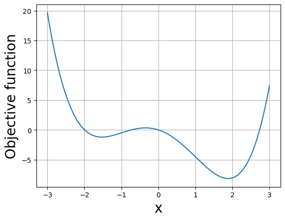
We now compare vanilla gradient descent to momentum-based gradient descent for a one-dimensional problem. This problem contains that persistent optimization goblin we all fear: the local minimum (cue scary sound effects). Note: the only way to get really good at coding is to add sound effects while you code—experimentally verified.

The objective function for this example is

(8.93)\[\begin{equation} \Phi(x) = \frac{1}{2}x^4 - 0.005x^3 - 3x^2 - 2x. \end{equation}\]

def objective(x):
    # Slight variation on Cornell's original function
    return 0.5*x**4 - 0.005*x**3 - 3*x**2 - 2*x

# Define the objective function
def objective(x):
    # Slight variation on Cornell's original function
    # Original: 0.3*x**4 - 0.1*x**3 - 2*x**2 - 0.8*x
    return 0.5*x**4 - 0.005*x**3 - 3*x**2 - 2*x

# Sample points
xmin=-3
xmax=3
nx=1000
x=jnp.linspace(xmin, xmax, nx) 

Phi = objective(x)

# Plot the objective function
fig, ax = plt.subplots()
ax.plot(x, Phi)
ax.set_xlabel("x", size=20)
ax.set_ylabel("Objective function", size=20)
ax.grid(True)
plt.show()

import jax
import jax.numpy as jnp
import numpy as np
from jax import grad

def gradient_descent(Phi, x0, n_iter, alpha, tol):
    """
    Vanilla gradient descent using JAX.

    Parameters
    ----------
    Phi : function
        Objective function to minimize.
    x0 : float
        Initial guess.
    n_iter : int
        Maximum number of iterations.
    alpha : float
        Learning rate.
    tol : float
        Tolerance for convergence.

    Returns
    -------
    x_data : np.ndarray
        Array of iterates.
    Phi(x_data[-1]) : float
        Objective function value at final iterate.
    """
    
    # Initialize storage for iterates
    x_data = np.full(n_iter, np.nan)
    x_data[0] = x0
    
    # JAX gradient
    dPhi = grad(Phi)
    
    for i in range(1, n_iter):
        g_i = dPhi(x0)          # compute gradient
        x = x0 - alpha * g_i    # update step
        x_data[i] = x
        
        if jnp.abs(x - x0) <= tol:
            print("Converged to", x)
            break
            
        x0 = x  # update current position
    
    # Remove unused entries
    x_data = x_data[~np.isnan(x_data)]
    
    return x_data, Phi(x_data[-1])

x0=-3.0

x1, sol1=gradient_descent(objective, x0, 200, .007, 1e-4) 

Converged to -1.5293782

import jax
import jax.numpy as jnp
import numpy as np
from jax import grad

def momentum_descent(Phi, x0, n_iter, mu, gamma, tol):
    """
    Gradient descent with momentum using JAX.

    Parameters
    ----------
    Phi : function
        Objective function to minimize.
    x0 : float
        Initial guess.
    n_iter : int
        Maximum number of iterations.
    mu : float
        Momentum coefficient (0 < mu < 1).
    gamma : float
        Learning rate.
    tol : float
        Tolerance for convergence.

    Returns
    -------
    x_data : np.ndarray
        Array of iterates.
    Phi(x_data[-1]) : float
        Objective function value at final iterate.
    """
    
    # Initialize storage for iterates
    x_data = np.full(n_iter, np.nan)
    x_data[0] = x0
    
    # Initialize momentum term
    b_i = 0.0
    
    # JAX gradient
    dPhi = grad(Phi)
    
    for i in range(1, n_iter):
        g_i = dPhi(x0)           # compute gradient
        b_i = mu * b_i + g_i     # update momentum
        x = x0 - gamma * b_i     # update position
        x_data[i] = x
        
        if jnp.abs(x - x0) <= tol:
            print("Converged to", x)
            break
            
        x0 = x  # update current position
    
    # Remove unused entries
    x_data = x_data[~np.isnan(x_data)]
    
    return x_data, Phi(x_data[-1])

x2, sol2= momentum_descent(objective, x0, 200, .7, 0.05, 1e-4) 

Converged to 1.8815817

# --- Run gradient descent methods ---
x0 = -3.0
n_iter = 50
alpha = 0.01
mu = 0.9
gamma = 0.01
tol = 1e-6

# x array for plotting the objective function
x = np.linspace(-3, 3, 400)
cost = objective(x)

# Compute iterates
x1, _ = gradient_descent(objective, x0, n_iter, alpha, tol)
x2, _ = momentum_descent(objective, x0, n_iter, mu, gamma, tol)

# Compute objective function values at all iterates
sol1 = objective(x1)
sol2 = objective(x2)

# --- Setup animation ---
n_frames = max(x1.size, x2.size)
n_stop = min(x1.size, x2.size)

fig = plt.figure(figsize=(10, 4))

# Vanilla gradient descent subplot
ax1 = fig.add_subplot(121)
ax1.set_title("Gradient Descent", size=20)
ax1.set_xlabel("x", size=20)
ax1.set_ylabel("Objective Function", size=20)
ax1.plot(x, cost, color='blue')
p1, = ax1.plot([], [], "o", color="red")
ax1.grid(True)

# Momentum gradient descent subplot
ax2 = fig.add_subplot(122)
ax2.set_title("Gradient Descent\nwith Momentum", size=20)
ax2.set_xlabel("x", size=20)
ax2.plot(x, cost, color='blue')
p2, = ax2.plot([], [], "o", color="red")
ax2.grid(True)

plt.tight_layout()
plt.close()

# Initialize animation
def init():
    p1.set_data([], [])
    p2.set_data([], [])
    return p1, p2

# Animation update function
def ani(i):
    if i >= n_stop:
        if x1.size < x2.size:
            p1.set_data([x1[n_stop-1]], [sol1[n_stop-1]])
            p2.set_data([x2[i]], [sol2[i]])
        else:
            p2.set_data([x2[n_stop-1]], [sol2[n_stop-1]])
            p1.set_data([x1[i]], [sol1[i]])
    else:
        p1.set_data([x1[i]], [sol1[i]])
        p2.set_data([x2[i]], [sol2[i]])
    return p1, p2

# Create the animation
anim = animation.FuncAnimation(fig, ani, frames=n_frames, init_func=init, interval=100, blit=True)

# To display in a Jupyter notebook
from IPython.display import HTML
HTML(anim.to_jshtml())

Once Loop Reflect

HTML(anim.to_html5_video())
anim.save("1D-momentum_gradient_descent.mp4")